Samacheer Kalvi 12th Business Maths Solutions Chapter 10 Operations Research Ex 10.1

Students can download 12th Business Maths Chapter 10 Operations Research Ex 10.1 Questions and Answers, Samacheer Kalvi 12th Business Maths Book Solutions Guide Pdf helps you to revise the complete Tamilnadu State Board New Syllabus and score more marks in your examinations.

Tamilnadu Samacheer Kalvi 12th Business Maths Solutions Chapter 10 Operations Research Ex 10.1

Question 1.
What is the transportation problem?
Solution:
The transportation problem deals with transporting goods from a source to a destination by minimum cost.
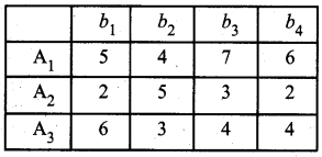
Description: A Manufacturer has a number of factories which produces goods at a fixed rate. He also has a number of warehouses, each of which has a fixed storage capacity. There is a cost to transport goods from a factory to a warehouse. Find the transportation of goods from factory to the warehouse that has the lowest possible cost.
Example:
Factories:
A1 makes 5 units
A2 makes 4 units
A3 makes 6 units
Warehouses:
b1 can store 5 units
b2 can store 3 units
b3 can store 5 units
b4 can store 2 units
Transportation costs:
Samacheer Kalvi 12th Business Maths Solutions Chapter 10 Operations Research Ex 10.1 1

Question 2.
Write the mathematical form of transportation problem.
Solution:
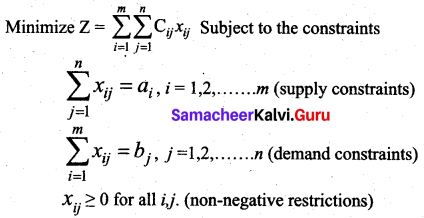
Mathematically a transportation problem is nothing but a special linear programming problem in which the objective function is to minimize the cost of transportation subjected to the demand and supply constraints.
Let there be ‘m’ sources of supply having ‘ai‘ units of supplies respectively to be transported among ‘n’ destinations with ‘bj‘ units of requirements respectively. Let Cij be the cost of shipping one unit of the commodity from source i to destination j for each route. Let xij be the units shipped per route.
Then the LPP is stated below.
Samacheer Kalvi 12th Business Maths Solutions Chapter 10 Operations Research Ex 10.1 2

Samacheer Kalvi 12th Business Maths Solutions Chapter 10 Operations Research Ex 10.1

Question 3.
What are a feasible solution and non-degenerate solution in the transportation problem?
Solution:
Feasible Solution: A feasible solution to a transportation problem is a set of non-negative values xij (i = 1, 2,.., m, j = 1, 2, …n) that satisfies the constraints.
Non-degenerate basic feasible Solution: If a basic feasible solution to a transportation problem contains exactly m + n – 1 allocation in independent positions, it is called a Non-degenerate basic feasible solution. Here m is the number of rows and n is the number of columns in a transportation problem.

Question 4.
What do you mean by balanced transportation problem?
Solution:
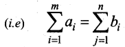
The balanced transportation problem is a transportation problem where the total availability at the origins is equal to the total requirements at the destinations.
Samacheer Kalvi 12th Business Maths Solutions Chapter 10 Operations Research Ex 10.1 3
A feasible solution can be obtained to these problems by Northwest comer method, minimum cost method (or) Vogel’s approximation method.

Samacheer Kalvi 12th Business Maths Solutions Chapter 10 Operations Research Ex 10.1

Question 5.
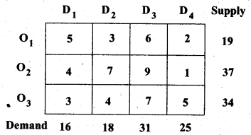
Find an initial basic feasible solution of the following problem using north-west corner rule.
Samacheer Kalvi 12th Business Maths Solutions Chapter 10 Operations Research Ex 10.1 4
Solution:
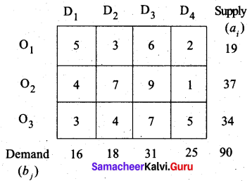
Given the transportation table is
Samacheer Kalvi 12th Business Maths Solutions Chapter 10 Operations Research Ex 10.1 5
Total supply = Total Demand = 90.
The given problem is a balanced transportation problem.
Hence there exists a feasible solution to the given problem.
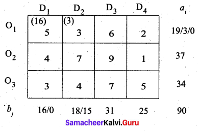
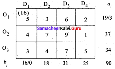
First allocation:
Samacheer Kalvi 12th Business Maths Solutions Chapter 10 Operations Research Ex 10.1 6
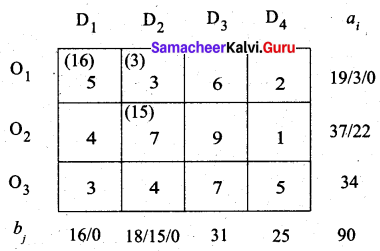
Second allocation:
Samacheer Kalvi 12th Business Maths Solutions Chapter 10 Operations Research Ex 10.1 73
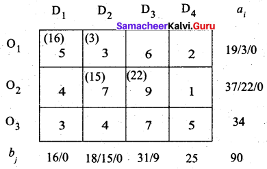
Third allocation:
Samacheer Kalvi 12th Business Maths Solutions Chapter 10 Operations Research Ex 10.1 7
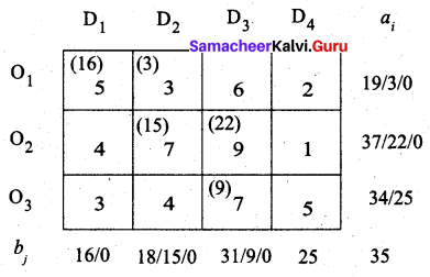
Fourth allocation:
Samacheer Kalvi 12th Business Maths Solutions Chapter 10 Operations Research Ex 10.1 8
Fifth allocation:
Samacheer Kalvi 12th Business Maths Solutions Chapter 10 Operations Research Ex 10.1 9
Final allocation:
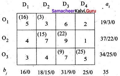
Samacheer Kalvi 12th Business Maths Solutions Chapter 10 Operations Research Ex 10.1 10
Transportation schedule:
O1 → D1, O1 → D2, O2 → D2, O2 → D3, O3 → D3, O3 → D4
(i.e) x11 = 16, x12 = 3, x22 = 15, x23 = 22, x33 = 9, x34 = 25.
Total transportation cost = (16 × 5) + (3 × 3) + (15 × 7) + (22 × 9) + (9 × 7) + (25 × 5)
= 80 + 9 + 105 + 198 + 63 + 125
= 580
Thus the minimum cost is Rs. 580 using the north west comer rule.

Samacheer Kalvi 12th Business Maths Solutions Chapter 10 Operations Research Ex 10.1

Question 6.
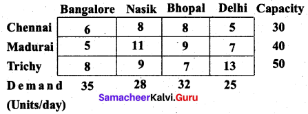
Determine an initial basic feasible solution of the following transportation problem by north-west corner method.
Samacheer Kalvi 12th Business Maths Solutions Chapter 10 Operations Research Ex 10.1 11
Solution:
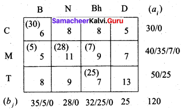
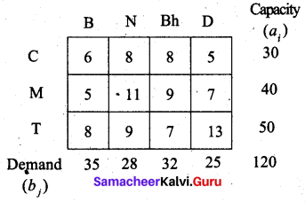
Let B, N, Bh, D represent the destinations Bangalore, Nasik, Bhopal and Delhi respectively.
Let C, M, T represent the starting places Chennai, Madurai and Trichy respectively.
The given transportation table is
Samacheer Kalvi 12th Business Maths Solutions Chapter 10 Operations Research Ex 10.1 12
Total capacity = Total Demand = 120.
So the given problem is a balanced transportation problem.
Hence there exists a feasible solution to the given problem.
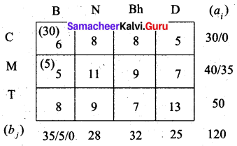
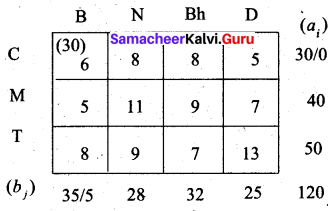
First allocation:
Samacheer Kalvi 12th Business Maths Solutions Chapter 10 Operations Research Ex 10.1 13
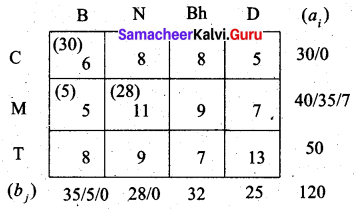
Second allocation:
Samacheer Kalvi 12th Business Maths Solutions Chapter 10 Operations Research Ex 10.1 14
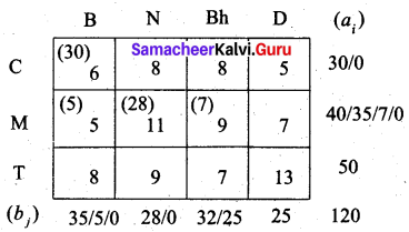
Third allocation:
Samacheer Kalvi 12th Business Maths Solutions Chapter 10 Operations Research Ex 10.1 15
Fourth allocation:
Samacheer Kalvi 12th Business Maths Solutions Chapter 10 Operations Research Ex 10.1 16
Fifth allocation:
Samacheer Kalvi 12th Business Maths Solutions Chapter 10 Operations Research Ex 10.1 17
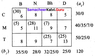
Final allocation:
Samacheer Kalvi 12th Business Maths Solutions Chapter 10 Operations Research Ex 10.1 18
Transportation schedule:
Chennai to Bangalore, Madurai to Bangalore, Madurai to Nasik, Madurai to Bhopal, Trichy to Bhopal, Trichy to Delhi.
(i.e) x11 = 30, x21 = 5, x22 = 28, x23 = 7, x33 = 25, x34 = 25
The total transportation cost = (30 × 6) + (5 × 5) + (28 × 11) + (7 × 9) + (25 × 7) + (25 × 13)
= 180 + 25 + 308 + 63 + 175 + 325
= 1076
Thus the minimum cost is Rs. 1076 by the north west comer method.

Question 7.
Obtain an initial basic feasible solution to the following transportation problem by using the least-cost method.
Samacheer Kalvi 12th Business Maths Solutions Chapter 10 Operations Research Ex 10.1 19
Solution:
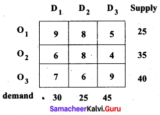
Total supply = 25 + 35 + 40 = 100
Total demand = 30 + 25 + 45 = 100
Total supply = Total demand
∴ The given problem is a balanced transportation problem. Hence there exists a feasible solution to the given problem. Let ‘ai’ denote the supply and ‘bj’ denote the demand. We allocate the units according to the least transportation cost of each cell.
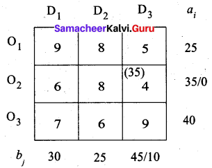
First allocation:
Samacheer Kalvi 12th Business Maths Solutions Chapter 10 Operations Research Ex 10.1 20
The least-cost 4 corresponds to cell (O2, D3). So first we allocate to this cell.
Second allocation:
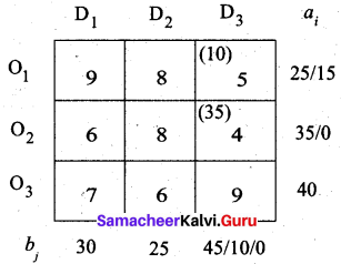
Samacheer Kalvi 12th Business Maths Solutions Chapter 10 Operations Research Ex 10.1 21
The least-cost 5 corresponds to cell (O1, D3). So we have allocated min (10, 25) to this cell.
Third allocation:
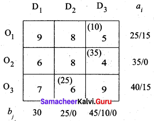
Samacheer Kalvi 12th Business Maths Solutions Chapter 10 Operations Research Ex 10.1 22
The least-cost 6 corresponds to cell (O3, D2). So we have allocated min (25, 40) to this cell.
Fourth allocation:
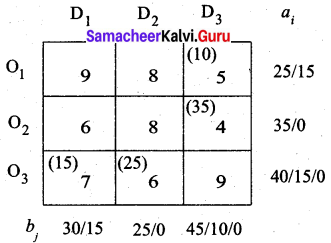
Samacheer Kalvi 12th Business Maths Solutions Chapter 10 Operations Research Ex 10.1 23
The least-cost 7 corresponds to cell (O3, D1). So we have allocated min (30, 15) to this cell.
Final allocation:
Although the next least cost is 8, we cannot allocate to cells (O1, D2) and (O2, D2) because we have exhausted the demand 25 for this column. So we allocate 15 to cell (O1, D1)
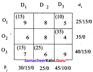
Samacheer Kalvi 12th Business Maths Solutions Chapter 10 Operations Research Ex 10.1 24
Transportation schedule: O1 → D1, O1 → D3, O2 → D3, O3 → D1, O3 → D2
(i.e) x11 = 15, x13 = 10, x23 = 35, x31 = 15, x32 = 25
Total cost is = (15 × 9) + (10 × 5) + (35 × 4) + (15 × 7) + (25 × 6)
= 135 + 50 + 140 + 105 + 150
= 580
Thus by least cost method (LCM) the cost is Rs. 580.

Samacheer Kalvi 12th Business Maths Solutions Chapter 10 Operations Research Ex 10.1

Question 8.
Explain Vogel’s approximation method by obtaining an initial feasible solution of the following transportation problem
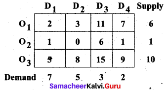
Samacheer Kalvi 12th Business Maths Solutions Chapter 10 Operations Research Ex 10.1 25
Solution:
Let ‘ai‘ denote the supply and ‘bj‘ denote the demand Σai = 6 + 1 + 10 = 17 and Σbj = 7 + 5 + 3 + 2 = 17
Σai = Σbj (i.e) Total supply = Total demand. the given problem is a balanced transportation problem. Hence there exists a feasible solution to the given problem.
First, we find the difference (penalty) between the first two smallest costs in each row and column and write them in brackets against the respective rows and columns.
First allocation:
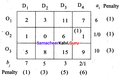
Samacheer Kalvi 12th Business Maths Solutions Chapter 10 Operations Research Ex 10.1 26
The largest difference is 6 corresponding to column D4. In this column least cost is (O2, D4). Allocate min (2, 1) to this cell.
Second allocation:
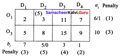
Samacheer Kalvi 12th Business Maths Solutions Chapter 10 Operations Research Ex 10.1 27
The largest difference is 5 in column D2. Here the least cost is (O1, D2). So allocate min (5, 6) to this cell.
Third allocation:
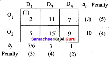
Samacheer Kalvi 12th Business Maths Solutions Chapter 10 Operations Research Ex 10.1 28
The largest penalty is 5 in row O1. The least cost is in (O1, D1). So allocate min (7, 1) here.
Fourth allocation:
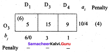
Samacheer Kalvi 12th Business Maths Solutions Chapter 10 Operations Research Ex 10.1 29
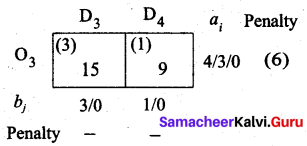
Fifth allocation:
Samacheer Kalvi 12th Business Maths Solutions Chapter 10 Operations Research Ex 10.1 30
We allocate min (1, 4) to (O3, D4) cell since it has the least cost. Finally the balance we allot to cell (O3, D3).
Thus we have the following allocations:
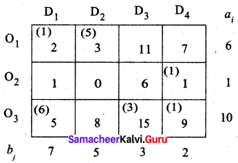
Samacheer Kalvi 12th Business Maths Solutions Chapter 10 Operations Research Ex 10.1 31
Transportation schedule:
O1 → D1, O1 → D2, O2 → D4, O3 → D1, O3 → D3, O3 → D4
(i.e) x11 = 12, x12 = 5, x24 = 1, x31 = 6, x33 = 3, x34 = 1
Total cost = (1 × 2) + (5 × 3) + (1 × 1) + (6 × 5) + (3 × 15) + (1 × 9)
= 2 + 15 + 1 + 30 + 45 + 9
= 102

Question 9.
Consider the following transportation problem.
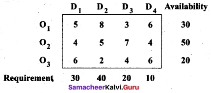
Samacheer Kalvi 12th Business Maths Solutions Chapter 10 Operations Research Ex 10.1 32
Determine initial basic feasible solution by VAM
Solution:
Let ‘ai‘ denote the availability and ’bj‘ denote the requirement
Σai = 30 + 50 + 20 = 100 and Σbj = 30 + 40 + 20 + 10 = 100
Σai = Σbj So the given problem is a balanced transportation problem. Hence there exists a feasible solution to the given problem.
For VAM, we first find the penalties for rows and columns. We allocate units to the maximum penalty column (or) row with the least cost.
First allocation:
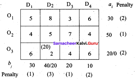
Samacheer Kalvi 12th Business Maths Solutions Chapter 10 Operations Research Ex 10.1 33
Largest penalty = 3. allocate min (40, 20) to (O3, D2)
Second allocation:
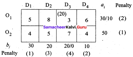
Samacheer Kalvi 12th Business Maths Solutions Chapter 10 Operations Research Ex 10.1 34
Largest penalty = 4. Allocate min (20, 30) to (O1, D3)
Third allocation:
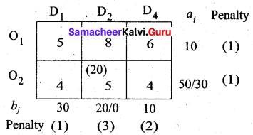
Samacheer Kalvi 12th Business Maths Solutions Chapter 10 Operations Research Ex 10.1 35
The largest penalty is 3. Allocate min (20, 50) to (O2, D2)
Fourth allocation:
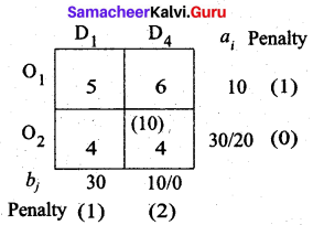
Samacheer Kalvi 12th Business Maths Solutions Chapter 10 Operations Research Ex 10.1 36
The largest penalty is 2, Allocate min (10, 30) to (O2, D4)
Fifth allocation:
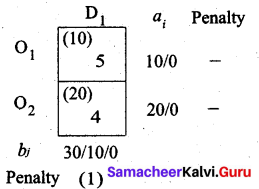
Samacheer Kalvi 12th Business Maths Solutions Chapter 10 Operations Research Ex 10.1 37
The largest penalty is 1. Allocate min (30, 20) to (O2, D1)
Balance 10 units we allot to (O1, D1).
Thus we have the following allocations:
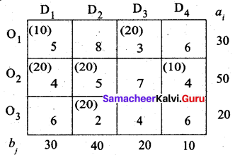
Samacheer Kalvi 12th Business Maths Solutions Chapter 10 Operations Research Ex 10.1 38
Transportation schedule:
O1 → D1, O1 → D3, O2 → D1, O2 → D2, O2 → D4, O3 → P2
(i.e) x11 = 10, x13 = 20, x21 = 20, x22 = 20, x24 = 10, x32 = 20
Total cost = (10 × 5) + (20 × 3) + (20 × 4) + (20 × 5) + (10 × 4) + (20 × 2)
= 50 + 60 + 80 + 100 + 40 + 40
= 370
Thus the least cost by YAM is Rs. 370.

Samacheer Kalvi 12th Business Maths Solutions Chapter 10 Operations Research Ex 10.1

Question 10.
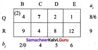
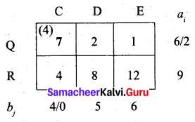
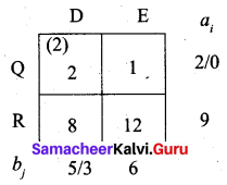
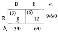
Determine the basic feasible solution to the following transportation problem using North West Corner rule.
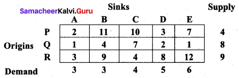
Samacheer Kalvi 12th Business Maths Solutions Chapter 10 Operations Research Ex 10.1 39
Solution:
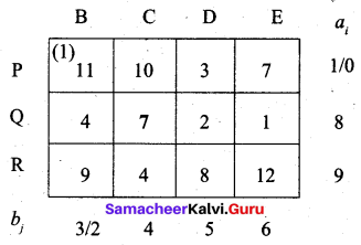
For the given problem, total supply is 4 + 8 + 9 = 21 and total demand is 3 + 3 + 4 + 5 + 6 = 21.
Since the total supply equals total demand, it is a balanced problem and we can find a feasible solution by North West Comer rule.
First allocation:
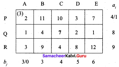
Samacheer Kalvi 12th Business Maths Solutions Chapter 10 Operations Research Ex 10.1 40
Second allocation:
Samacheer Kalvi 12th Business Maths Solutions Chapter 10 Operations Research Ex 10.1 41
Third allocation:
Samacheer Kalvi 12th Business Maths Solutions Chapter 10 Operations Research Ex 10.1 42
Fourth allocation:
Samacheer Kalvi 12th Business Maths Solutions Chapter 10 Operations Research Ex 10.1 43
Fifth allocation:
Samacheer Kalvi 12th Business Maths Solutions Chapter 10 Operations Research Ex 10.1 44
Final allocation:
Samacheer Kalvi 12th Business Maths Solutions Chapter 10 Operations Research Ex 10.1 45
First, we allow 3 units to (R, D) cell. Then balance 6 to (R, E) cell.
Thus we have the following allocations:
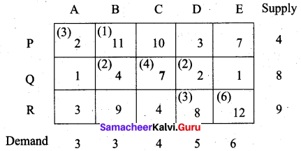
Samacheer Kalvi 12th Business Maths Solutions Chapter 10 Operations Research Ex 10.1 46
Transportation schedule:
P → A, P → B, Q → B, Q → C, Q → D, R → D, R → E
(i.e) x11 = 3, x12 = 1, x22 = 2, x23 = 4, x24 = 2, x34 = 3, x35 = 6
Total cost = (3 × 2) + (1 × 11) + (2 × 4) + (4 × 7) + (2 × 2) + (3 × 8) + (6 × 12)
= 6 + 11 + 8 + 28 + 4 + 24 + 72
= 153
Thus the minimum cost of the transportation problem by Northwest Comer rule is Rs. 153.

Samacheer Kalvi 12th Business Maths Solutions Chapter 10 Operations Research Ex 10.1

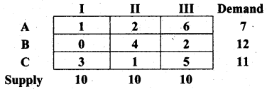
Question 11.
Find the initial basic feasible solution of the following transportation problem:
Samacheer Kalvi 12th Business Maths Solutions Chapter 10 Operations Research Ex 10.1 47
Using (i) North West Corner rule
(ii) Least Cost method
(iii) Vogel’s approximation method
Solution:
Total demand (ai) = 7 + 12 + 11 = 30 and total supply (bj) = 10 + 10 + 10 = 30.
Σai = Σbj ⇒ the problem is a balanced transportation problem and we can find a basic feasible solution.
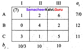
(i) North West Comer rule (NWC)
First allocation:
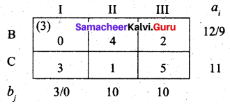
Samacheer Kalvi 12th Business Maths Solutions Chapter 10 Operations Research Ex 10.1 48
Second allocation:
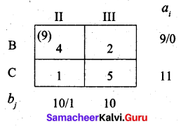
Samacheer Kalvi 12th Business Maths Solutions Chapter 10 Operations Research Ex 10.1 49
Third allocation:
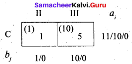
Samacheer Kalvi 12th Business Maths Solutions Chapter 10 Operations Research Ex 10.1 50
Fourth allocation:
Samacheer Kalvi 12th Business Maths Solutions Chapter 10 Operations Research Ex 10.1 51
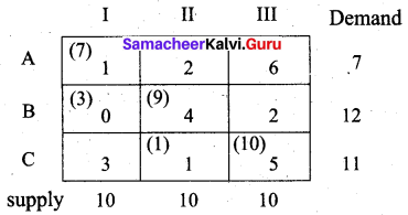
We first allot 1 unit to (C, II) cell and then the balance 10 units to (C, III) cell.
Thus we have the following allocations:
Samacheer Kalvi 12th Business Maths Solutions Chapter 10 Operations Research Ex 10.1 52
Transportation schedule:
A → I, B → I, B → II, C → II, C → III
(i.e) x11 = 7, x21 = 3, x22 = 9, x32 = 1, x33 = 10
Total cost = (7 × 1) + (3 × 0) + (9 × 4) + (1 × 1) + (10 × 5)
= 7 + 0 + 36 + 1 + 50
= Rs. 94

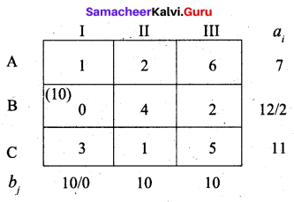
(ii) Least Cost method
First allocation:
Samacheer Kalvi 12th Business Maths Solutions Chapter 10 Operations Research Ex 10.1 53
Second allocation:
Samacheer Kalvi 12th Business Maths Solutions Chapter 10 Operations Research Ex 10.1 54
Third allocation:
Samacheer Kalvi 12th Business Maths Solutions Chapter 10 Operations Research Ex 10.1 55
Fourth allocation:
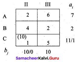
Samacheer Kalvi 12th Business Maths Solutions Chapter 10 Operations Research Ex 10.1 56
We first allot 1 unit to cell (C, III) and the balance 7 units to cell (A, III).
Thus we have the following allocations:
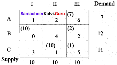
Samacheer Kalvi 12th Business Maths Solutions Chapter 10 Operations Research Ex 10.1 57
Transportation schedule:
A → III, B → I, B → III, C → II, C → III
(i.e) x13 = 7, x21 = 10, x23 = 2, x32 = 10, x33 = 1
Total cost = (7 × 6) + (10 × 0) + (2 × 2) + (10 × 1) + (1 × 5)
= 42 + 0 + 4 + 10 + 5
= Rs. 61

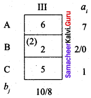
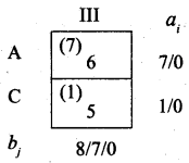
(iii) Vogel’s approximation method (VAM)
First allocation:
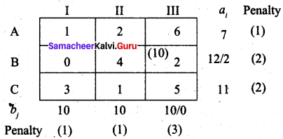
Samacheer Kalvi 12th Business Maths Solutions Chapter 10 Operations Research Ex 10.1 58
Largest penalty = 3. Allocate min (10, 12) to (B, III)
Second allocation:
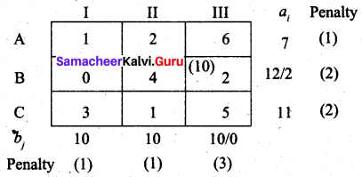
Samacheer Kalvi 12th Business Maths Solutions Chapter 10 Operations Research Ex 10.1 59
Largest penalty = 4. Allocate min (10, 2) to cell (B, I)
Third allocation:
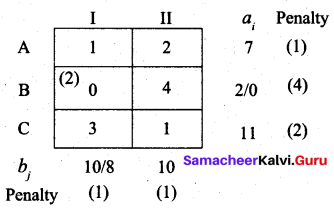
Samacheer Kalvi 12th Business Maths Solutions Chapter 10 Operations Research Ex 10.1 60
The largest penalty is 2. We can choose I column or C row. Allocate min (8, 7) to cell (A, I)
Fourth allocation:
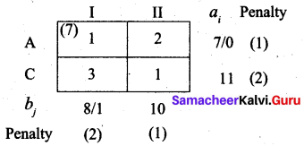
Samacheer Kalvi 12th Business Maths Solutions Chapter 10 Operations Research Ex 10.1 61
First, we allocate 10 units to cell (C, II). Then balance 1 unit we allot to cell (C, I)
Thus we have the following allocations:
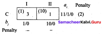
Samaacheer Kalvi 12th Business Maths Solutions Chapter 10 Operations Research Ex 10.1 62
TYansportation schedule:
A → I, B → I, B → III, C → I, C → II
(i.e) x11 = 7, x21 = 2, x23 = 10, x31 = 1, x32 = 10
Total cost = (7 × 1) + (2 × 0) + (10 × 2) + (1 × 3) + (10 × 1)
= 7 + 0 + 20 + 3 + 10
= Rs. 40

Samacheer Kalvi 12th Business Maths Solutions Chapter 10 Operations Research Ex 10.1

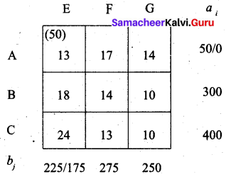
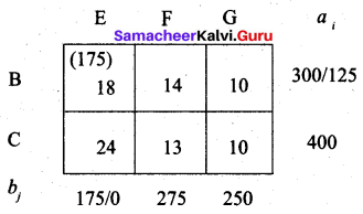
Question 12.
Obtain an initial basic feasible solution to the following transportation problem by north-west corner method.
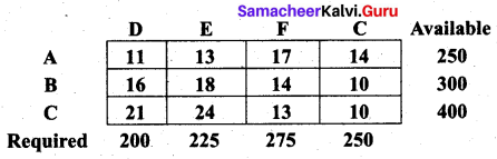
Samaacheer Kalvi 12th Business Maths Solutions Chapter 10 Operations Research Ex 10.1 63
Solution:
Total availability is 250 + 300 + 400 = 950
Total requirement is 200 + 225 + 275 + 250 = 950
Since Σai = Σbj the problem is a balanced transportation problem and we can find an initial basic feasible solution.
First Allocation:
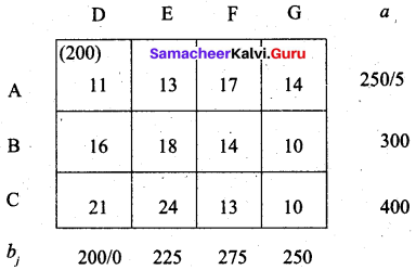
Samaacheer Kalvi 12th Business Maths Solutions Chapter 10 Operations Research Ex 10.1 64
Second allocation:
Samaacheer Kalvi 12th Business Maths Solutions Chapter 10 Operations Research Ex 10.1 65
Third allocation:
Samaacheer Kalvi 12th Business Maths Solutions Chapter 10 Operations Research Ex 10.1 66
Fourth allocation:
Samaacheer Kalvi 12th Business Maths Solutions Chapter 10 Operations Research Ex 10.1 67
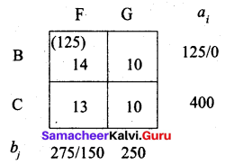
Fifth allocation:
Samaacheer Kalvi 12th Business Maths Solutions Chapter 10 Operations Research Ex 10.1 68
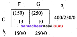
We first allocate 150 units to cell (C, F). Then we allocate balance of 250 units to cell (C, G)
Thus we have the following allocation.
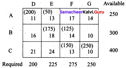
Samaacheer Kalvi 12th Business Maths Solutions Chapter 10 Operations Research Ex 10.1 69
Transportation schedule:
A → D, A → E, B → E, B → F, C → F, C → G
(i.e) x11 = 200, x12 = 50, x22 = 175, x23 = 125, x33 = 150, x34 = 250
Total cost = (200 × 11) + (50 × 13) + (175 × 18) + (125 × 14) + (150 × 13) + (250 × 10)
= 2200 + 650 + 3150 + 1750 + 1950 + 2500
= Rs. 12,200
Samacheer Kalvi 12th Business Maths Solutions Chapter 9 Applied Statistics Ex 9.1

Students can download 12th Business Maths Chapter 9 Applied Statistics Ex 9.1 Questions and Answers, Samacheer Kalvi 12th Business Maths Book Solutions Guide Pdf helps you to revise the complete Tamilnadu State Board New Syllabus and score more marks in your examinations.

Tamilnadu Samacheer Kalvi 12th Business Maths Solutions Chapter 9 Applied Statistics Ex 9.1

Question 1.
Define Time series.
Solution:
When quantitative data are arranged in the order of their occurrence, the resulting series is called the Time Series.

Question 2.
What is the need for studying time series?
Solution:
We should study time series for the following reasons.

  • It helps in the analysis of past behaviour.
  • It helps in forecasting and for future plans.
  • It helps in the evaluation of current achievements.
  • It helps in making comparative studies between one time period and others.

Therefore time series helps us to study and analyze the time-related data which involves in business fields, economics, industries, etc…

Samacheer Kalvi 12th Business Maths Solutions Chapter 9 Applied Statistics Ex 9.1

Question 3.
State the uses of time series.
Solution:
A time-series carries profound importance in business and policy planning. It is used to compare the current trends with that in the past or the expected trends. Thus it gives a clear picture of growth or downfall. Most of the time series data related to fields like Economics, Business, Commerce etc. For example the production of a product, cost of a product, sales of a product, national income, salary of an individual etc. By close observation of time series data, one can predict and plan for future operations in industries and other fields.

Question 4.
Mention the components of the time series.
Solution:
Components of Time Series
There are four types of components in a time series. They are as follows;

  1. Secular Trend
  2. Seasonal variations
  3. Cyclic variations
  4. Irregular variations

Samacheer Kalvi 12th Business Maths Solutions Chapter 9 Applied Statistics Ex 9.1

Question 5.
Define the secular trend.
Solution:
Secular Trend: It is a general tendency, of time series to increase or decrease or stagnates during a long period of time. An upward tendency is usually observed in the population of a country, production, sales, prices in industries, the income of individuals etc., A downward tendency is observed in deaths, epidemics, prices of electronic gadgets, water sources, mortality rate etc….

Question 6.
Write a brief note on seasonal variations.
Solution:
Seasonal Variations: As the name suggests, tendency movements are due to nature which repeats themselves periodically in every season. These variations repeat themselves in less than one year time. It is measured in an interval of time. Seasonal variations may be influenced by natural force, social customs and traditions. These variations are the results of such factors which uniformly and regularly rise and fall in the magnitude. For example, selling of umbrellas’ and raincoat in the rainy season, sales of cool drinks in the summer season, crackers in Deepawali season, purchase of dresses in a festival season, sugarcane in Pongal season.

Samacheer Kalvi 12th Business Maths Solutions Chapter 9 Applied Statistics Ex 9.1

Question 7.
Explain cyclic variations.
Solution:
Cyclic Variations: These variations are not necessarily uniformly periodic in nature. That is, they may or may not follow exactly similar patterns after equal intervals of time. Generally, one cyclic period ranges from 7 to 9 years and there is no hard and fast rule in the fixation of years for a cyclic period. For example, every business cycle has a Start- Boom-Depression- Recover, maintenance during booms and depressions, changes in government monetary policies, changes in interest rates.

Question 8.
Discuss irregular variation.
Solution:
Irregular Variations: These variations do not have a particular pattern and there is no regular period of time of their occurrences. These are accidental changes which are purely random or unpredictable. Normally they are short – term variations, but its occurrence sometimes has its effect so intense that they may give rise to new cyclic or other movements of variations. For example floods, wars, earthquakes, Tsunami, strikes, lockouts etc…

Samacheer Kalvi 12th Business Maths Solutions Chapter 9 Applied Statistics Ex 9.1

Question 9.
Define the seasonal index.
Solution:
Seasonal Index for every season (i.e) months, quarters or year is given by
Seasonal Index (S.I) = \(\frac{\text { Seasonal Average }}{\text { Grand average }}\) × 100
Where seasonal average is calculated for month, (or) quarter depending on the problem and Grand Average (G) is the average of averages.

Question 10.
Explain the method of fitting a straight line.
Solution:
The method of fitting a straight line is as follows
Procedure:
(i) The straight-line trend is represented by the equation Y = a + bX ….. (1)
where Y is the actual value, X is time, a, b are constants
(ii) The constants ‘a’ and ‘b’ are estimated by solving the following two normal Equations
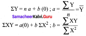
ΣY = n a + b ΣX ……(2)
ΣXY = a ΣX + b ΣX2 ……(3)
Where n = number of years given in the data.
(iii) By taking the mid-point of the time as the origin, we get ΣX = 0
(iv) When ΣX = 0, the two normal equations reduces to
Samacheer Kalvi 12th Business Maths Solutions Chapter 9 Applied Statistics Ex 9.1 Q10
The constant ‘a’ gives the mean of Y and ‘6’ gives the rate of change (slope).
(v) By substituting the values of ‘a’ and ‘b’ in the trend equation (1), we get the Line of Best Fit.

Samacheer Kalvi 12th Business Maths Solutions Chapter 9 Applied Statistics Ex 9.1

Question 11.
State the two normal equations used in fitting a straight line.
Solution:
The normal equations used in fitting a straight line are
ΣY = na + b ΣX and ΣXY = a ΣX + b ΣX2
Where n = number of years given in the data,
X = time
Y = actual value
a, b = constants

Question 12.
State the different methods of measuring trend.
Solution:
Measurements of Trends
Following are the methods by which we can measure the trend.

  1. Freehand or Graphic Method
  2. Method of Semi-Averages
  3. Method of Moving Averages
  4. Method of Least Squares

Samacheer Kalvi 12th Business Maths Solutions Chapter 9 Applied Statistics Ex 9.1

Question 13.
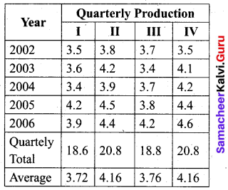
Compute the average seasonal movement for the following series.
Samacheer Kalvi 12th Business Maths Solutions Chapter 9 Applied Statistics Ex 9.1 Q13
Solution:
Samacheer Kalvi 12th Business Maths Solutions Chapter 9 Applied Statistics Ex 9.1 Q13.1
Grand average = \(\frac{3.72+4.16+3.76+4.16}{4}\) = 3.95
Seasonal Index (S.I) for I quarter = \(\frac { Average\quad of\quad I\quad quarter }{ Grand\quad Average }\) × 100
S.I. for I quarter = \(\frac{3.72}{3.95}\) × 100 = 94.1772
S.I. for II quarter = \(\frac{4.16}{3.95}\) × 100 = 105.3165
S.I. for III quarter = \(\frac{3.76}{3.95}\) × 100 = 95.1899
S.I. for IV quarter = \(\frac{4.16}{3.95}\) × 100 = 105.3165
Thus we obtain the average seasonal movement.

Question 14.
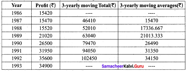
The following figures relate to the profits of a commercial concern for 8 years.
Samacheer Kalvi 12th Business Maths Solutions Chapter 9 Applied Statistics Ex 9.1 Q14
Find the trend of profits by the method of three year moving averages.
Solution:
Computation of three-yearly moving averages
Samacheer Kalvi 12th Business Maths Solutions Chapter 9 Applied Statistics Ex 9.1 Q14.1
The last column gives the trend of profits.

Samacheer Kalvi 12th Business Maths Solutions Chapter 9 Applied Statistics Ex 9.1

Question 15.
Find the trend of production by the method of a five-yearly period of moving average for the following data:
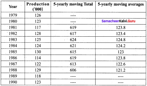
Samacheer Kalvi 12th Business Maths Solutions Chapter 9 Applied Statistics Ex 9.1 Q15
Solution:
Computation of five-yearly moving averages
Samacheer Kalvi 12th Business Maths Solutions Chapter 9 Applied Statistics Ex 9.1 Q15.1
The last column gives the trend in the production by the method of the five-yearly period of moving average.

Question 16.
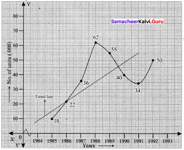
The following table gives the number of small – scale units registered with the Directorate of Industries between 1985 and 1991. Show the growth on a trend line by the freehand method.
Samacheer Kalvi 12th Business Maths Solutions Chapter 9 Applied Statistics Ex 9.1 Q16
Solution:
We follow the procedure as given below
(a) Plot the data on a graph
(b) Join all the points by a free hand smooth curve
(c) A line is drawn which passes through the maximum number of plotted points
Samacheer Kalvi 12th Business Maths Solutions Chapter 9 Applied Statistics Ex 9.1 Q16.1

Samacheer Kalvi 12th Business Maths Solutions Chapter 9 Applied Statistics Ex 9.1

Question 17.
The Annual production of a commodity is given as follows:
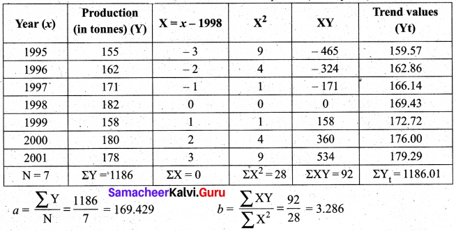
Samacheer Kalvi 12th Business Maths Solutions Chapter 9 Applied Statistics Ex 9.1 Q17
Fit a straight line trend by the method of least squares.
Solution:
Computation of trend values by the method of least squares. (ODD years)
Samacheer Kalvi 12th Business Maths Solutions Chapter 9 Applied Statistics Ex 9.1 Q17.1
Therefore, the required equation of the straight line trend is given by Y = a + bX
(i.e) Y = 169.429 + 3.286 X (or) Y = 169.429 + 3.286 (x – 1998)
The trends values are obtained by
When x = 1995, Yt = 169.429 + 3.286 (1995 – 1998) = 159.57
When x = 1996, Yt = 169.429 + 3.286 (1996 – 1998) = 162.86
When x = 1997, Yt = 169.429 + 3.286 (1997 – 1998) = 166.14
When x = 1998, Yt = -169.429 + 3.286 (1998 – 1998) = 169.43
When x = 1999, Yt = 169.429 + 3.286 (1999 – 1998) = 172:72
When x = 2000, Yt = 169.429 + 3.286 (2000 – 1998) = 176.00
When x = 2001, Yt = 169.429 + 3.286 (2001 – 1998) = 179.29

Question 18.
Determine the equation of a straight line which best fits the following data.
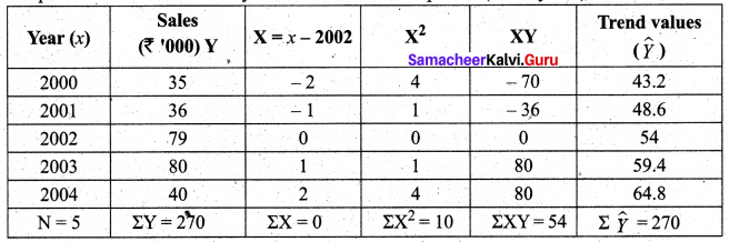
Samacheer Kalvi 12th Business Maths Solutions Chapter 9 Applied Statistics Ex 9.1 Q18
Compute the trend values for all years from 2000 to 2004.
Solution:
Computation of trend values by the method of least squares. (ODD years)
Samacheer Kalvi 12th Business Maths Solutions Chapter 9 Applied Statistics Ex 9.1 Q18.1
Samacheer Kalvi 12th Business Maths Solutions Chapter 9 Applied Statistics Ex 9.1 Q18.2
Therefore, the equation of the straight line which best fits the data is given by Y = a + b X
(i.e) Y= 54 + 5.4 X
(or) Y = 54 + 5.4 (x – 2002)
The trends values are obtained as follows
When x = 2000, \(\hat{Y}\) = 54 + 5.4 (2000 – 2002) = 43.2
When x = 2001, \(\hat{Y}\) = 54 + 5.4 (2001 – 2002) = 48.6
When x = 2002, \(\hat{Y}\) = 54 + 5.4 (2002 – 2002) = 54
When x = 2003, \(\hat{Y}\) = 54 + 5.4 (2003 – 2002) = 59.4
When x = 2004, \(\hat{Y}\) = 54 + 5.4 (2004 – 2002) = 64.8

Samacheer Kalvi 12th Business Maths Solutions Chapter 9 Applied Statistics Ex 9.1

Question 19.
The sales of a commodity in tones varied from January 2010 to December 2010 as follows:
Samacheer Kalvi 12th Business Maths Solutions Chapter 9 Applied Statistics Ex 9.1 Q19
Fit a trend line by the method of semi-average.
Solution:
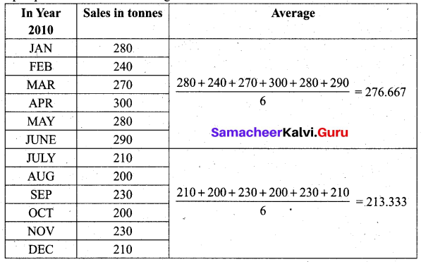
Since the number of months is even (12), we can equally divide the given data in two equal parts and obtain the averages of the first six months and last six months
Samacheer Kalvi 12th Business Maths Solutions Chapter 9 Applied Statistics Ex 9.1 Q19.1
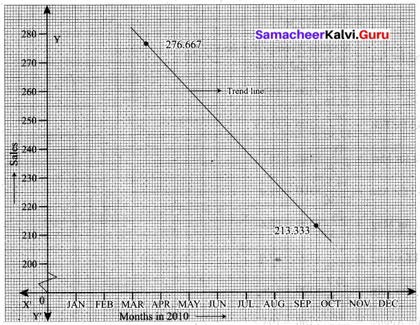
Thus we obtain semi-average I = 276.667 and semi-average II = 213.333
To fit a trend line we plot each value at the mid-point (month) of each half, (i.e) we plot 276.667 in the middle of March and April; we plot 213.333 in the middle of September and October. We join the two points by a straight line. This is the required line.
Samacheer Kalvi 12th Business Maths Solutions Chapter 9 Applied Statistics Ex 9.1 Q19.2

Question 20.
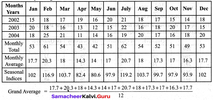
Use the method of monthly averages to find the monthly indices for the following data of production of a commodity for the years 2002, 2003 and 2004.
Samacheer Kalvi 12th Business Maths Solutions Chapter 9 Applied Statistics Ex 9.1 Q20
Solution:
Computation of monthly indices for the production of a commodity using the method of monthly averages.
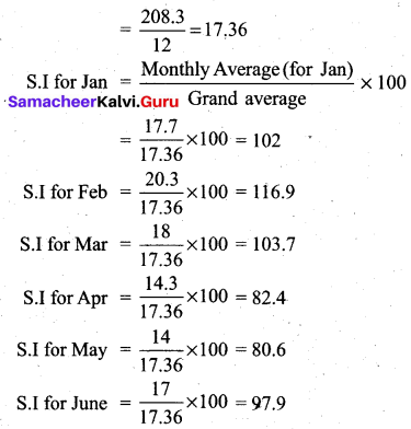
Samacheer Kalvi 12th Business Maths Solutions Chapter 9 Applied Statistics Ex 9.1 Q20.1
Samacheer Kalvi 12th Business Maths Solutions Chapter 9 Applied Statistics Ex 9.1 Q20.2
Samacheer Kalvi 12th Business Maths Solutions Chapter 9 Applied Statistics Ex 9.1 Q20.3
All the values are given in the above table in the last row.

Samacheer Kalvi 12th Business Maths Solutions Chapter 9 Applied Statistics Ex 9.1

Question 21.
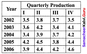
Calculate the seasonal indices from the following data using the average from the following data using the average method:
Samacheer Kalvi 12th Business Maths Solutions Chapter 9 Applied Statistics Ex 9.1 Q21
Solution:
Computation of quarterly indices.by the method of simple averages.
Samacheer Kalvi 12th Business Maths Solutions Chapter 9 Applied Statistics Ex 9.1 Q21.1
Samacheer Kalvi 12th Business Maths Solutions Chapter 9 Applied Statistics Ex 9.1 Q21.2
The seasonal indices are given in the last row of the table above.

Question 22.
The following table shows the number of salesmen working for a certain concern.
Samacheer Kalvi 12th Business Maths Solutions Chapter 9 Applied Statistics Ex 9.1 Q22
Use the method of least squares to fit a straight line and estimate the number of salesmen in 1997.
Solution:
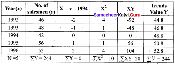
Samacheer Kalvi 12th Business Maths Solutions Chapter 9 Applied Statistics Ex 9.1 Q22.1
Samacheer Kalvi 12th Business Maths Solutions Chapter 9 Applied Statistics Ex 9.1 Q22.2
Therefore, the required equation of the straight line trend is given by
Y = a + bX
Y = 48.8 + 2 X
Y = 48.8 + 2 (x – 1994)
The trend values are obtained as follows:
When x = 1992, \(\hat{Y}\) = 48.8 + 2(1992 – 1994) = 44.8
When x = 1993, \(\hat{Y}\) = 48.8 + 2 (1993 – 1994) = 46.8
When x = 1994, \(\hat{Y}\) = 48.8 + 2 (1994 – 1994) = 48.8
When x = 1995, \(\hat{Y}\) = 48.8 + 2 (1995 – 1994) = 50.8
When x = 1996, \(\hat{Y}\) = 48.8 + 2 (1996 – 1994) = 52.8
In the year 1997, the estimated number of salesmen is \(\hat{Y}\) = 48.8 + 2 (1997 – 1994)
= 48.8 + 6
= 54.8 ~ 55

Samacheer Kalvi 12th Business Maths Solutions Chapter 7 Probability Distributions Miscellaneous Problems

Students can download 12th Business Maths Chapter 7 Probability Distributions Miscellaneous Problems and Answers, Samacheer Kalvi 12th Business Maths Book Solutions Guide Pdf helps you to revise the complete Tamilnadu State Board New Syllabus and score more marks in your examinations.

Tamilnadu Samacheer Kalvi 12th Business Maths Solutions Chapter 7 Probability Distributions Miscellaneous Problems

Question 1.
A manufacturer of metal pistons finds that on the average, 12% of his pistons are rejected because they are either oversize or undersize. What is the probability that a batch of 10 pistons will contain
(a) no more than 2 rejects?
(b) at least 2 rejects?
Solution:
Let X be the binomial random variable denoting the number of metal pistons.
Let p be the probability of rejections.
Given that p = 12% = \(\frac{12}{100}\) = 0.12, q = 0.88, n = 10.
So X ~ B(0.12, 10). Hence the p.m.f of X is given by
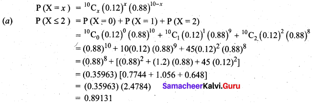
Samacheer Kalvi 12th Business Maths Solutions Chapter 7 Probability Distributions Miscellaneous Problems Q1
Thus out of a batch of 10 pistons, the probability of no more than 2 rejects is 0.89131
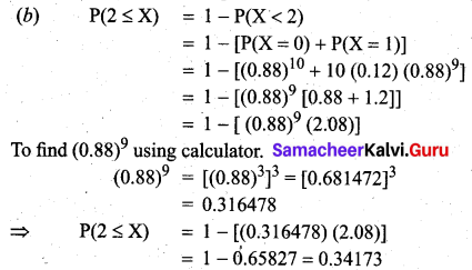
Samacheer Kalvi 12th Business Maths Solutions Chapter 7 Probability Distributions Miscellaneous Problems Q1.1
Thus out of 10 pistons, the probability that at least 2 will be rejected is 0.34173

Question 2.
Hospital records show that of patients suffering from a certain disease 75% die of it. What is the probability that of 6 randomly selected patients, 4 will recover?
Solution:
Let X be the binomial random variable denoting the number of patients.
Let p be the probability that the patient will recover and q be the probability that patient will die.
According to the problem, q = 75% = 0.75 and p = 25% = 0.25 and n = 6
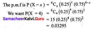
Samacheer Kalvi 12th Business Maths Solutions Chapter 7 Probability Distributions Miscellaneous Problems Q2
Hence the probability that 4 patients will recover out of 6 patients is 0.03295

Samacheer Kalvi 12th Business Maths Solutions Chapter 7 Probability Distributions Miscellaneous Problems

Question 3.
If electricity power failures occur according to a Poisson distribution with an average of 3 failures every twenty weeks, calculate the probability that there will not be more than one failure during a particular week.
Solution:
Let X be the poisson random variable. It is given that mean λ = \(\frac{3}{20}\) = 0.15
The Poisson probability law, giving x failures per week is given by,
Samacheer Kalvi 12th Business Maths Solutions Chapter 7 Probability Distributions Miscellaneous Problems Q3
Hence probability that there will not be more than one failure is given by P (X ≤ 1)
= P(X = 0) + P(X = 1)
= e-0.15 [1 + 0.15]
= e-0.15 (1.15)
= (0.8607) (1.15)
= 0.98981

Question 4.
Vehicles pass through a junction on a busy road at an average rate of 300 per hour.
(а) Find the probability that none passes in a given minute.
(b) What is the expected number passing in two minutes?
Solution:
Let X be the Poisson random variable. It is given that mean
λ = 300/hour = 300/60 minutes = 5 per minute.
(a) The Poisson law giving x vehicles passing on a road in one minute is given by
Samacheer Kalvi 12th Business Maths Solutions Chapter 7 Probability Distributions Miscellaneous Problems Q4
Now the probability that no vehicles pass in a given minute is given by,
Samacheer Kalvi 12th Business Maths Solutions Chapter 7 Probability Distributions Miscellaneous Problems Q4.1
(b) E(X) = λ (i.e) No of vehicles passing per minute, since λ = 5, the expected number passing in two minutes is 10.

Samacheer Kalvi 12th Business Maths Solutions Chapter 7 Probability Distributions Miscellaneous Problems

Question 5.
Entry to a certain University is determined by a national test. The scores on this test are normally distributed with a mean of 500 and a standard deviation of 100. Raghul wants to be admitted to this university and he knows that he must score better than at least 70% of the students who took the test. Raghul takes the test and scores 585. Will he be admitted to this university?
Solution:
Let X be the normal random variable denoting the scores of the students. Given that mean µ = 500 and s.d σ = 100. The total area under the normal curve represents the total number of students who took the test. If we multiply the values of the areas under the curve by 100, we obtain percentages.
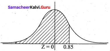
Samacheer Kalvi 12th Business Maths Solutions Chapter 7 Probability Distributions Miscellaneous Problems Q5
When X = 585, Z = \(\frac{585-500}{100}\) = 0.85
The proportion of students who scored below 585 is given by P[area to the left of Z = 0.85]
(i.e.) P (Z < 0.85) = 0.5 + P (0 < Z < 0.85)
= 0.5 + 0.3023 .
= 0.8023
= 80.23%
Raghul scored better than 80.23% of the students who took the test and he will be admitted to this university.

Question 6.
The time taken to assemble a car in a certain plant is a random variable having a normal distribution of 20 hours and a standard deviation of 2 hours. What is the probability that a car can be assembled at this plant in a period of time?
(a) less than 19.5 hours?
(b) between 20 and 22 hours?
Solution:
Let X be the normal random variable denoting the time taken to assemble a car.
Given that mean µ = 20 and s.d σ = 2
(a) Probability that car is assembled in less than 19.5 hours
P(X < 19.5) = P(Z < \(\frac{19.5-20}{2}\))
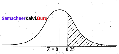
P(Z < -0.25) = P(Z > 0.25)
= 0.5 – P(0 < Z < 0.25)
= 0.5 – 0.0987
= 0.4013
Samacheer Kalvi 12th Business Maths Solutions Chapter 7 Probability Distributions Miscellaneous Problems Q6
(b) The probability that a car can be assembled between 20 and 22 hours is given by
P(20 < X < 22) = P(\(\frac{20-20}{2}\) < Z < \(\frac{22-20}{2}\))
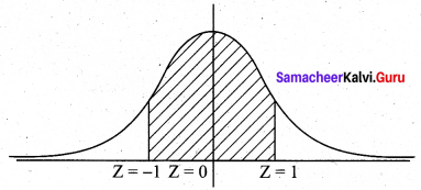
P(0 < Z < 1) = 0.3413

Samacheer Kalvi 12th Business Maths Solutions Chapter 7 Probability Distributions Miscellaneous Problems

Question 7.
The annual salaries of employees in a large company are approximately normally distributed with a mean of $50,000 and a standard deviation of $20,000.
(а) What per cent of people earn less than $ 40,000?
(b) What per cent of people earn between $ 45,000 and $65,000?
(c) What per cent of people*earn more than $ 70,000?
Solution:
Let X be the normal variable denoting the annual salaries of employees.
Given the mean µ = 50,000 and s.d σ = 20,000
(a) Probability of people ehming less than $ 40,000 is given by P (X < 40,000)
= P(X < 40,000)
= P(Z < \(\frac{40000-50000}{20,000}\))
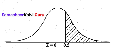
= P (Z < -0.5)
= P (0.5 < Z) (By symmetry)
= 0.5 – P(0 < Z < 0.5)
= 0.5 – 0.1915
= 0.3085
Hence people who earn less than $40,000 is 0.3085 × 100 = 30.85%
Samacheer Kalvi 12th Business Maths Solutions Chapter 7 Probability Distributions Miscellaneous Problems Q7
(b) Probability of people earning between $45,000 and $65,000 is P(45000 < X < 65000)
= P(\(\frac{45000-50000}{20000}\) < Z < \(\frac{65000-50000}{20000}\))
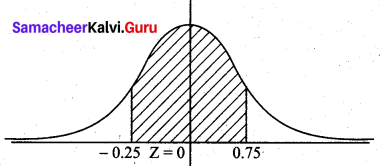
= P (-0.25 < Z < 0.75)
= P(-0.25 < Z < 0) + P (0 < Z < 0.75)
= P(0 < Z < 0.25) + P (0 < Z < 0.75)
= 0.0987 + 0.2734
= 0.3721
Hence percent of people who earn between $45,000 and $65,000 is 0.3721 × 100 = 37.21%
Samacheer Kalvi 12th Business Maths Solutions Chapter 7 Probability Distributions Miscellaneous Problems Q7.1
(c) Probability of people earning more than $ 70,000 is P(X > 70,000)
= P(Z > \(\frac{70000-50000}{20000}\))
= P(Z > 1)
= 0.5 – P(0 < Z < 1)
= 0.5 – 0.3413
= 0.1587
Hence percent of people who earn more than $70,000 is 0.1587 × 100 = 15.87%
Samacheer Kalvi 12th Business Maths Solutions Chapter 7 Probability Distributions Miscellaneous Problems Q7.2

Question 8.
X is a normally distributed variable with mean µ = 30 and standard deviation σ = 4. Find
(a) P(X < 40) (b) P(X > 21)
(c) P(30 < X < 35).
Solution:
Given X ~ N (µ, σ2)
µ = 30, σ = 4
(a) P(X < 40) = P(Z < \(\frac{40-30}{4}\))
= P(Z < 2.5)
= 0.5 + P(0 < Z < 2.5)
= 0.5 + 0.4938
= 0.9938
Samacheer Kalvi 12th Business Maths Solutions Chapter 7 Probability Distributions Miscellaneous Problems Q8
(b) P(X > 21) = P(Z > \(\frac{21-30}{4}\))
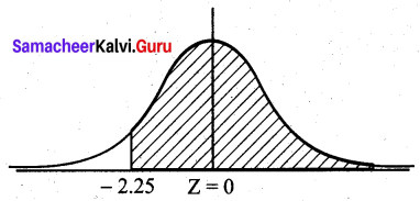
= P (Z > -2.25)
= 0.5 + P(-2.25 < Z < 0)
= 0 5 + P (0 < Z < 2.25)
= 0.5 + 0.4878
= 0.9878
Samacheer Kalvi 12th Business Maths Solutions Chapter 7 Probability Distributions Miscellaneous Problems Q8.1
(c) P(30 < X < 35)
= P(\(\frac{30-30}{4}\) < Z < \(\frac{35-30}{4}\))
= P(0 < Z < 1.25)
= 0.3944

Samacheer Kalvi 12th Business Maths Solutions Chapter 7 Probability Distributions Miscellaneous Problems

Question 9.
The birth weight of babies is normally distributed with mean 3,500g and standard deviation 500g, What is the probability that a baby is born that weight less than 3,100g?
Solution:
Let X be the normal variable denoting the birth weights of babies. Given that the mean µ = 3500 and s.d σ = 500
Samacheer Kalvi 12th Business Maths Solutions Chapter 7 Probability Distributions Miscellaneous Problems Q9
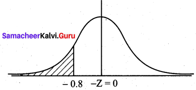
Probability that a baby is bom with weight less than 3100 g = P (X < 3100)
= P(Z < \(\frac{3100-3500}{500}\))
= P (Z < -0.8) = P (Z > 0.8) (by symmetry)
= 0.5 – P(0 < Z < 0.8)
= 0.5 – 0.2881
= 0.2119

Question 10.
People’s monthly electric bills in Chennai are normally distributed with a mean of ₹ 225 and a standard deviation of ₹ 55. Those people spend a lot of time online. In a group of 500 customers, how many would we expect to have a bill that is ₹ 100 or less?
Solution:
Let X be the normal variable denoting the monthly bills in rupees.
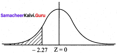
Samacheer Kalvi 12th Business Maths Solutions Chapter 7 Probability Distributions Miscellaneous Problems Q10
Given mean µ = 225 and s.d σ = 55
Now the probability that the bill will be ₹100 or less is P (X ≤ 100)
= P(Z ≤ \(\frac{100-225}{55}\))
= P(Z ≤ -2.27)
= 0.5 – P(-2.27 < Z < 0)
= 0.5 – P(0 < Z < 2.27)
= 0.5 – 0.4884
= 0.0116
Thus, in a group of 500 customers, we expect to have 500 × 0.0116 = 5.8 ~ 6 customers whose electric bills will be ₹ 100 or less.

Samacheer Kalvi 12th Business Maths Solutions Chapter 7 Probability Distributions Ex 7.4

Students can download 12th Business Maths Chapter 7 Probability Distributions Ex 7.4 Questions and Answers, Samacheer Kalvi 12th Business Maths Book Solutions Guide Pdf helps you to revise the complete Tamilnadu State Board New Syllabus and score more marks in your examinations.

Tamilnadu Samacheer Kalvi 12th Business Maths Solutions Chapter 7 Probability Distributions Ex 7.4

Choose the correct answer:

Question 1.
Normal distribution was invented by ______
(a) Laplace
(b) De-Moivre
(c) Gauss
(d) all the above
Answer:
(b) De-Moivre

Question 2.
If X ~ N (9, 81) the standard normal variate Z will be ______
(a) Z = \(\frac{x-81}{9}\)
(b) Z = \(\frac{X-9}{81}\)
(c) Z = \(\frac{X-9}{9}\)
(d) Z = \(\frac{9-x}{9}\)
Answer:
(c) Z = \(\frac{X-9}{9}\)
Hint:
µ = 9, σ = 9
Z = \(\frac{X-9}{9}\)

Samacheer Kalvi 12th Business Maths Solutions Chapter 7 Probability Distributions Ex 7.4

Question 3.
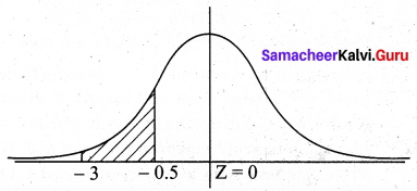
If Z is a standard normal variate, the proportion of items lying between Z = -0.5 and Z = -3.0 is ________
(a) 0.4987
(b) 0.1915
(c) 0.3072
(d) 0.3098
Answer:
(c) 0.3072
Hint:
Samacheer Kalvi 12th Business Maths Solutions Chapter 7 Probability Distributions Ex 7.4 Q3
P(-0.5 < Z < -3)
By symmetry we want P (0.5 < Z < 3)
= P(0 < Z < 3) – P(0 < Z < 0.5)
= 0.49865 – 0.1915
= 0.30715 ~ 0.3072

Question 4.
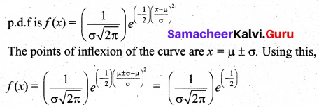
If X ~ N(µ, σ2), the maximum probability at the point of inflexion of normal distribution is ______
(a) \(\left(\frac{1}{\sqrt{2 \pi}}\right) e^{\frac{1}{2}}\)
(b) \(\left(\frac{1}{\sqrt{2 \pi}}\right) e^{\left(-\frac{1}{2}\right)}\)
(c) \(\left(\frac{1}{\sigma \sqrt{2 \pi}}\right) e^{\left(-\frac{1}{2}\right)}\)
(d) \(\left(\frac{1}{\sqrt{2 \pi}}\right)\)
Answer:
(c) \(\left(\frac{1}{\sigma \sqrt{2 \pi}}\right) e^{\left(-\frac{1}{2}\right)}\)
Hint:
Samacheer Kalvi 12th Business Maths Solutions Chapter 7 Probability Distributions Ex 7.4 Q4

Question 5.
In a parametric distribution the mean is equal to variance is ________
(a) binomial
(b) normal
(c) Poisson
(d) all of the above
Answer:
(c) Poisson

Samacheer Kalvi 12th Business Maths Solutions Chapter 7 Probability Distributions Ex 7.4

Question 6.
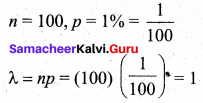
In turning out certain toys in a manufacturing company, the average number of defectives is 1%. The probability that the sample of 100 toys there will be 3 defectives is __________
(a) 0.0613
(b) 0.613
(c) 0.00613
(d) 0.3913
Answer:
(a) 0.0613
Hint:
Samacheer Kalvi 12th Business Maths Solutions Chapter 7 Probability Distributions Ex 7.4 Q6
Samacheer Kalvi 12th Business Maths Solutions Chapter 7 Probability Distributions Ex 7.4 Q6.1

Question 7.
The parameters of the normal distribution f(x) = \(\frac{1}{\sqrt{72 \pi}} \frac{e^{(-x-10)^{2}}}{72}-\infty<x<\infty\)
(a) (10, 6)
(b) (10, 36)
(c) (6, 10)
(d) (36, 10)
Answer:
(b) (10, 36)
Hint:
Comparing f(x) with p.d.f of normal distribution, µ = 10,
\(\sigma \sqrt{2 \pi}=\sqrt{72 \pi}=\sqrt{36 \times 2 \pi}=6 \sqrt{2 \pi}\)
σ = 6

Samacheer Kalvi 12th Business Maths Solutions Chapter 7 Probability Distributions Ex 7.4

Question 8.
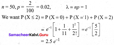
A manufacturer produces switches and experiences that 2 per cent switches are defective. The probability that in a box of 50 switches, there are at most two defective is:
(a) 2.5 e-1
(b) e-1
(c) 2e-1
(d) none of the above
Answer:
(a) 2.5 e-1
Hint:
Samacheer Kalvi 12th Business Maths Solutions Chapter 7 Probability Distributions Ex 7.4 Q8

Question 9.
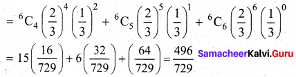
An experiment succeeds twice as often as it fails. The chance that in the next six trials, there shall be at least four successes is _______
(a) \(\frac {240}{729}\)
(b) \(\frac {489}{729}\)
(c) \(\frac {496}{729}\)
(d) \(\frac {251}{729}\)
Answer:
(c) \(\frac {496}{729}\)
Hint:
Let X be the binomial random variable. Given p = 2q
From p + q = 1 ,we get p = \(\frac{2}{3}\), q = \(\frac{1}{3}\)
We want P(X ≥ 4) = P(X = 4) + P(X = 5) + P(X = 6)
Samacheer Kalvi 12th Business Maths Solutions Chapter 7 Probability Distributions Ex 7.4 Q9

Question 10.
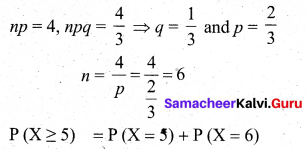
If for a binomial distribution b(n, p) mean = 4 and variance = \(\frac{4}{3}\), the probability, P(X ≥ 5) is equal to _______
(a) (2/3)6
(b) (2/3)5 (1/3)
(c) (1/3)6
(d) 4(2/3)6
Answer:
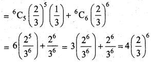
(d) 4(2/3)6
Hint:
Samacheer Kalvi 12th Business Maths Solutions Chapter 7 Probability Distributions Ex 7.4 Q10
Samacheer Kalvi 12th Business Maths Solutions Chapter 7 Probability Distributions Ex 7.4 Q10.1

Question 11.
The average percentage of failure in a certain examination is 40. The probability that out of a group of 6 candidates atleast 4 passed in the examination are _______
(a) 0.5443
(b) 0.4543
(c) 0.5543
(d) 0.4573
Answer:
(a) 0.5443
Hint:
The percentage of success p = 0.6 ⇒ q = 0.4
P (X ≥ 4) = P (X = 4) + P (X = 5) + P (X = 6)
Samacheer Kalvi 12th Business Maths Solutions Chapter 7 Probability Distributions Ex 7.4 Q11
= 0.31104 + 0.186624 + 0.046656
= 0.54432

Samacheer Kalvi 12th Business Maths Solutions Chapter 7 Probability Distributions Ex 7.4

Question 12.
Forty per cent of the passengers who fly on a certain route do not check in any luggage. The planes on this route seat 15 passengers. For a full flight, what is the mean of the number of passengers who do not check in any luggage?
(a) 6.00
(b) 6.45
(c) 7.20
(d) 7.50
Answer:
(a) 6.00
Hint:
n = 15, p = 0.4 ⇒ mean (np) = 6

Question 13.
Which of the following statements is/are true regarding the normal distribution curve?
(а) it is a symmetrical and bell-shaped curve
(b) it is asymptotic in that each end approaches the horizontal axis but never reaches it
(c) its mean, median and mode are located at the same point
(d) all of the above statements are true
Answer:
(d) all of the above statements are true

Samacheer Kalvi 12th Business Maths Solutions Chapter 7 Probability Distributions Ex 7.4

Question 14.
Which of the following cannot generate a Poisson distribution?
(а) The number of telephone calls received in a ten-minute interval
(b) The number of customers arriving at a petrol station
(c) The number of bacteria found in a cubic foot of soil
(d) The number of misprints per page
Answer:
(b) The number of customers arriving at a petrol station

Question 15.
The random variable X is normally distributed with a mean of 70 and a standard deviation of 10. What is the probability that X is between 72 and 84?
(a) 0.683
(b) 0.954
(c) 0.271
(d) 0.340
Answer:
(d) 0.340
Hint:
µ = 70, σ = 10
P(72 < X < 84) = P(\(\frac{72-70}{10}\) < Z < \(\frac{84-70}{10}\))
= P(0.2 < Z < 1.4)
= P(0 < Z < 1.4) – P(0 < Z < 0.2)
= 0.4192 – 0.0793
= 0.3399
= 0.340

Samacheer Kalvi 12th Business Maths Solutions Chapter 7 Probability Distributions Ex 7.4

Question 16.
The starting annual salaries of newly qualified chartered accountants (CA’s) in South Africa follow a normal distribution with a mean of ₹ 180,000 and a standard deviation of ₹ 10,000. What is the probability that a randomly selected newly qualified CA will earn between ₹ 165,000 and ₹ 175,000.
(a) 0.819
(b) 0.242
(c) 0.286
(d) 0.533
Answer:
(b) 0.242
Hint:
Samacheer Kalvi 12th Business Maths Solutions Chapter 7 Probability Distributions Ex 7.4 Q16
µ = 180,000, σ = 10,000
P(165,000 < X < 175,000)
= P(\(\frac{165,000-180,000}{10,000}\) < Z < \(\frac{175,000-180,000}{10,000}\))
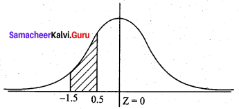
= P(-1.5 < Z < -0.5)
By symmetry of the normal curve,
= P (0.5 < Z < 1.5)
= P (0 < Z < 1.5) – P(0 < Z < 0.5)
= 0.4332 – 0.1915
= 0.2417
= 0.242

Question 17.
In a large statistics class the heights of the students are normally distributed with a mean of 172 cm and a variance of 25 cm. What proportion of students are between 165cm and 181 cm in height?
(a) 0.954
(b) 0.601
(c) 0.718
(d) 0.883
Answer:
(d) 0.883
Hint:
Samacheer Kalvi 12th Business Maths Solutions Chapter 7 Probability Distributions Ex 7.4 Q17
µ = 172, σ2 = 25 ⇒ σ = 5
P (165 < X < 181)
= P(\(\frac{165-172}{5}\) < Z < \(\frac{181-172}{5}\))
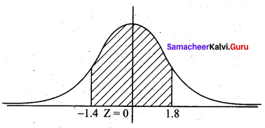
= P(-1.4 < Z < 1.8)
= P (-1.4 < Z < 0) + P(0 < Z < 1.8)
= P(0 < Z < 1.4) + P(0 < Z < 1.8)
= 0.4192 + 0.4641
= 0.8833

Samacheer Kalvi 12th Business Maths Solutions Chapter 7 Probability Distributions Ex 7.4

Question 18.
A statistical analysis of long-distance telephone calls indicates that the length of these calls is normally distributed with a mean of 240 seconds and a standard deviation of 40 seconds. What proportion of calls lasts less than 180 seconds?
(a) 0.214
(b) 0.094
(c) 0.933
(d) 0.067
Answer:
(d) 0.067
Hint:
Samacheer Kalvi 12th Business Maths Solutions Chapter 7 Probability Distributions Ex 7.4 Q18
µ = 240, σ = 40
P(X < 180)
= P(Z < \(\frac{180-240}{40}\))
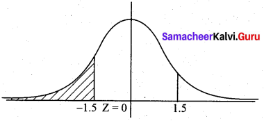
= P(Z < -1.5) = P(Z > 1.5)
= 0.5 – P (0 < Z < 1.5)
= 0.5 – 0.4332
= 0.0668
= 0.067

Question 19.
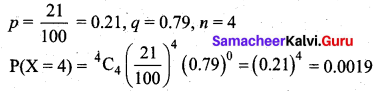
Cape town is estimated to have 21% of homes whose owners subscribe to the satellite service, DSTV. If a random sample of your home in taken, what is the probability that all four home subscribe to DSTV?
(a) 0.2100
(b) 0.5000
(c) 0.8791
(d) 0.0019
Answer:
(d) 0.0019
Hint:
Samacheer Kalvi 12th Business Maths Solutions Chapter 7 Probability Distributions Ex 7.4 Q19

Question 20.
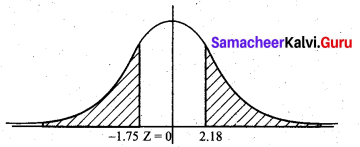
Using the standard normal table, the sum of the probabilities to the right of z = 2.18 and to the left of z = -1.75 is:
(a) 0.4854
(b) 0.4599
(c) 0.0146
(d) 0.0547
Answer:
(d) 0.0547
Hint:
Samacheer Kalvi 12th Business Maths Solutions Chapter 7 Probability Distributions Ex 7.4 Q20
P(Z > 2.18) + P(Z < -1.75)
= 0.5 – P(0 < Z < 2.18) + P (Z > 1.75)
= 0.5 – P(0 < Z < 2.18) + 0.5 – P(0 < Z < 1.75)
= 0.5 – 0.4854 + 0.5 – 0.4599
= 0.0547

Samacheer Kalvi 12th Business Maths Solutions Chapter 7 Probability Distributions Ex 7.4

Question 21.
The time until first failure of a brand of inkjet printers is normally distributed with a mean of 1,500 hours and a standard deviation of 200 hours. What proportion of printers fails before 1000 hours?
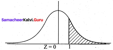
(a) 0.0062
(b) 0.0668
(c) 0.8413
(d) 0.0228
Answer:
(a) 0.0062
Hint:
µ = 1500, σ = 200
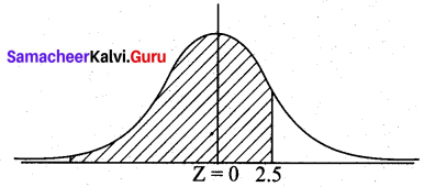
P(X < 1000)
= P(Z < \(\frac{1000-1500}{200}\))
= P(Z < -2.5) = P (Z > 2.5)
= 0.5 – P (0 < Z < 2.5)
= 0.5 – 0.4938
= 0.0062

Question 22.
The weights of newborn human babies are normally distributed with a mean of 3.2 kg and a standard deviation of 1.1 kg. What is the probability that a randomly selected newborn baby weight less than 2.0 kg?
(a) 0.138
(b) 0.428
(c) 0.766
(d) 0.262
Answer:
(a) 0.138
Hint:
µ = 3.2, σ = 1.1
P (X < 2)
= P( Z < \(\frac{2-3.2}{1.1}\))
= P(Z < -1.09) = P(Z > 1.09)
= 0.5 – P(0 < Z < 1.09)
= 0.5 – 0.3621
= 0.138

Samacheer Kalvi 12th Business Maths Solutions Chapter 7 Probability Distributions Ex 7.4

Question 23.
Monthly expenditure on their credit cards, by credit card holders from a certain bank, follows a normal distribution with a mean of ₹ 1,295.00 and a standard deviation of ₹ 750.00. What proportion of credit card holders spend more than ₹ 1,500.00 on their credit cards per month?
(a) 0.487
(b) 0.394
(c) 0.500
(d) 0.791
Answer:
(b) 0.394
Hint:
µ = 1295, σ = 750
P(X > 1500)
= P(Z > \(\frac{1500-1295}{750}\))
= P (Z > 0.27)
= 0.5 – P (0 < Z < 0.27)
= 0.5 – 0.1064
= 0.3936 ~ 0.394

Question 24.
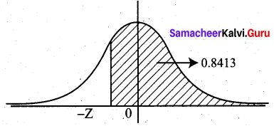
Let z be a standard normal variable. If the area to the right of z is 0.8413, then the value of z must be:
(a) 1.00
(b) -1.00
(c) 0.00
(d) -0.41
Answer:
(b) -1.00
Hint:
Samacheer Kalvi 12th Business Maths Solutions Chapter 7 Probability Distributions Ex 7.4 Q24
P(Z > -Z) = 0.8413
⇒ P(-z < Z < 0) + 0.5 = 0.8413
P(0 < Z < z) = 0.8413 – 0.5 = 0.3413
from normal tables, z = 1.
The required value is -z = -1

Samacheer Kalvi 12th Business Maths Solutions Chapter 7 Probability Distributions Ex 7.4

Question 25.
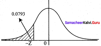
If the area to the left of a value of z (z has a standard normal distribution) is 0.0793, what is the value of z?
(a) -1.41
(b) 1.41.
(c) -2.25
(d) 2.25
Answer:
(a) -1.41
Hint:
Samacheer Kalvi 12th Business Maths Solutions Chapter 7 Probability Distributions Ex 7.4 Q25
P(Z < -z) = 0.0793 By symmetry, P (Z > z) = 0.0793
(i.e) 0.5 – P (0 < Z < z) = 0.0793
P(0 < Z < z) = 0.4207 from normal tables, z = 1.41
Thus the required value is -1.41 (since it is left of Z = 0)

Question 26.
If P(Z > z) = 0.8508 what is the value of z (z has a standard normal distribution)?
(a) -0.48
(b) 0.48
(c) -1.04
(d) -0.21
Answer:
(c) -1.04
Hint:
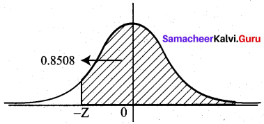
Samacheer Kalvi 12th Business Maths Solutions Chapter 7 Probability Distributions Ex 7.4 Q26
P (Z > z) = 0.8508
Since the given value is more than we take z to the left of Z = 0 axis.
P (Z > -z) = 0.8508
P(-z < Z < 0) + 0.5 = 0.8508
P(0 < Z < z) = 0.3508
From normal tables, z = 1.04
So required value is -1.04

Samacheer Kalvi 12th Business Maths Solutions Chapter 7 Probability Distributions Ex 7.4

Question 27.
If P(Z > z) = 0.5832 what is the value of z (z has a standard normal distribution)?
(a) -0.48
(b) 0.48
(c) 1.04
(d) -0.21
Answer:
(d) -0.21
Hint:
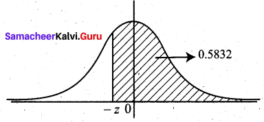
Samacheer Kalvi 12th Business Maths Solutions Chapter 7 Probability Distributions Ex 7.4 Q27
P(0 < Z < z) = 0.5832 – 0.5 = 0.0832
From tables, z = 0.21
Since z is to the left of Z = 0, the required value is -0.21

Question 28.
In a binomial distribution, the probability of success is twice as that of failure. Then out of 4 trials, the probability of no success is _______
(a) \(\frac {16}{81}\)
(b) \(\frac {1}{16}\)
(c) \(\frac {2}{27}\)
(d) \(\frac {1}{81}\)
Answer:
(d) \(\frac {1}{81}\)
Hint:
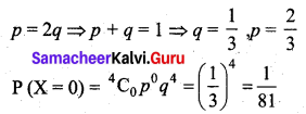
Samacheer Kalvi 12th Business Maths Solutions Chapter 7 Probability Distributions Ex 7.4 Q28

Samacheer Kalvi 12th Business Maths Solutions Chapter 8 Sampling Techniques and Statistical Inference Miscellaneous Problems

Students can download 12th Business Maths Chapter 8 Sampling Techniques and Statistical Inference Miscellaneous Problems and Answers, Samacheer Kalvi 12th Business Maths Book Solutions Guide Pdf helps you to revise the complete Tamilnadu State Board New Syllabus and score more marks in your examinations.

Tamilnadu Samacheer Kalvi 12th Business Maths Solutions Chapter 8 Sampling Techniques and Statistical Inference Miscellaneous Problems

Question 1.
Explain the types of sampling.
Solution:
The different types of sampling are

  • simple random sampling
  • Stratified random sampling and
  • Systematic sampling

(i) In simple random sampling, every item of the population has an equal chance for being selected. The sampling can be done with replacement (or) without replacement. A random sampling from a finite population with replacement is equivalent to sampling from an infinite population without replacement. This technique will give useful results only if the population is homogeneous. The following are some of the methods of selecting a random sample.

(a) Use of an unbiased die or coin: If we have to choose between two alternatives, a coin is tossed and depending on the head or tail course of action is taken. A die can be employed if there are six different alternatives.

(b) Lottery sampling: Here a random sample is selected by identifying each element of the population by means of a card of a pack of uniform cards or (by writing the number on pieces of paper) and to select a required number of cards after thorough mixing of the cards.

(c) Random numbers: Random numbers are formed of ‘random digits’ and arranged in the form of a table having a number of rows and columns. Tippett’s numbers form one such table wherein 40,000 digits were selected at random from census reports and combined by groups of four into 10,000 numbers.

(ii) In stratified random sampling, a population of units is divided into L sub-populations of N1, N2, …… NL. The sub-populations being non-overlapping and mutually exhaustive so that N = N1 + N2 + …….. + NL. Each sub-populations is known as a stratum. If we select n1, n2, ……. nl items, respectively, from these strata, we get a stratified sample. If a simple random sample is taken from each stratum, the whole procedure is referred to as stratified random sampling.

Samacheer Kalvi 12th Business Maths Solutions Chapter 8 Sampling Techniques and Statistical Inference Miscellaneous Problems

(iii) Systematic sampling is a form of restricted random selection which is highly useful in surveys concerning enumerable population. In this method, every member of the population is numbered in serial order and every ith element, starting from any of the first items is chosen. For example, suppose we require a 5% sample of students from a college where there are 2000 students, we select a random number from 1 to 20. If it is 12, then our sample consists of students with numbers 12, 32, 52, 72, …… 1992.

Question 2.
Write a short note on sampling distribution and standard error.
Solution:
Sampling distribution: Sampling distribution of a statistic is the frequency distribution which is formed with various values of a statistic computed from different samples of the same size drawn from the same population.
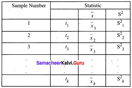
For instance if we draw a sample of size n from a given finite population of size N, then the total number of possible samples is \(^{\mathrm{N}} C_{n}=\frac{\mathrm{N} !}{n !(N-n) !}=k\) (say). For each of these k samples we can compute some statistic, t = t(x1, x2, x3 ,… xn), in particular the mean \(\bar{X}\) the variance S2, etc., is given below
Samacheer Kalvi 12th Business Maths Solutions Chapter 8 Sampling Techniques and Statistical Inference Miscellaneous Problems Q2
The set of the values of the statistic so obtained, one for each sample constitutes the sampling distribution of the statistic.

Samacheer Kalvi 12th Business Maths Solutions Chapter 8 Sampling Techniques and Statistical Inference Miscellaneous Problems

Standard Error:
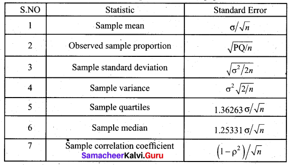
The standard deviation of the sampling distribution of a statistic is known as its Standard Error abbreviated as S.E. The Standard Errors (S.E.) of some of the well-known statistics, for large samples, are given below, where n is the sample size, σ2 is the population variance.
Samacheer Kalvi 12th Business Maths Solutions Chapter 8 Sampling Techniques and Statistical Inference Miscellaneous Problems Q2.1

Question 3.
Explain the procedures of testing of hypothesis.
Solution:
Hypothesis testing addresses the important question of how to choose among alternative propositions while controlling and minimizing the risk of wrong decisions. A hypothesis which is tested for possible rejection is called null hypothesis H0 and the hypothesis which is opposite to this is the alternative hypothesis H1. There are two basic types of decision problems that can be considered in a hypothesis testing procedure.
(a) whether a population parameter has changed from or differs from a particular value.
(b) whether the sample has come from the population that has a parameter value less than or more than the hypothesized value.

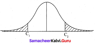
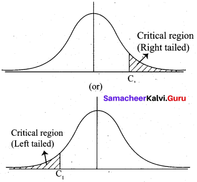
The set of all possible values of the sample statistic is referred to as the sample space. The test procedure divides the sample space into two parts called the acceptance region and rejection region (critical region). In the case of the two-tailed test, we find two values C1 and C2 which set the limits on the amount of sampling variation consistent with the null hypothesis H0. For the one-tailed test, we find only one value C1
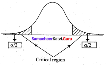
Samacheer Kalvi 12th Business Maths Solutions Chapter 8 Sampling Techniques and Statistical Inference Miscellaneous Problems Q3
When the hypothesis H0 is rejected when it is true the error is Type I error. When H0 is accepted when it is false it is called Type II error. When the calculated value of the test statistic is less than the table value, we accept the null hypothesis H0; otherwise, accept alternative hypothesis H1.
Samacheer Kalvi 12th Business Maths Solutions Chapter 8 Sampling Techniques and Statistical Inference Miscellaneous Problems Q3.1

Question 4.
Explain in detail about the test of significance of a single mean.
Solution:
A random sample of size n (n ≥ 30) is drawn from a population. We want to test the population mean has a specified value µ0.
Procedure for testing: (For two-tail test)
The null hypothesis is H0 : µ = µ0.
The alternative hypothesis is H1 : µ ≠ µ2
Since n is large the sampling distribution of \(\bar{x}\) (the sample mean) is approximately normal.
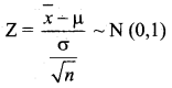
The test statistic
Samacheer Kalvi 12th Business Maths Solutions Chapter 8 Sampling Techniques and Statistical Inference Miscellaneous Problems Q4
For a significance level α = 0.05 (5% level)
If |Z| < 1.96, H0 is accepted at 5% level. If |Z| > 1.96, H0 is rejected at 5% level
For α = 0.01 (1% level), if |Z| < 2.58, H0 is accepted. If |Z| > 2.58, H0 is rejected.
Procedure for one tail test: (left tail)
H0 : µ ≥ µ0
H1 : µ < µ0
At α = 0.05, |Z| = 1.645
If Z < -1.645, H0 is rejected If Z > -1.645, H0 is accepted
One tail test: (right tail)
If Z < 1.645, H0 is accepted If Z > 1.645, H0 is rejected at 5% level of significance.

Samacheer Kalvi 12th Business Maths Solutions Chapter 8 Sampling Techniques and Statistical Inference Miscellaneous Problems

Question 5.
Determine the standard error of proportion for a random sample of 500 pineapples was taken from a large consignment and 65 were found to be bad.
Solution:
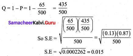
The standard error of proportion is S.E. = \(\sqrt{\mathrm{PQ} / \mathrm{n}}\)
Given sample size n = 500 and P = \(\frac{65}{500}\)
Samacheer Kalvi 12th Business Maths Solutions Chapter 8 Sampling Techniques and Statistical Inference Miscellaneous Problems Q5

Question 6.
A sample of 100 students is drawn from a school. The mean weight and variance of the sample are 67.45 kg and 9 kg. respectively. Find (a) 95% (b) 99% confidence intervals for estimating the mean weight of the students.
Solution:
Given Sample size n = 100
Sample mean \(\bar{x}\) = 67.45 kg
Sample S.D s = √9 = 3 kg
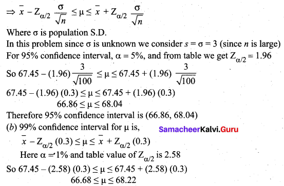
(a) 95% confidence interval for population mean µ is,
Samacheer Kalvi 12th Business Maths Solutions Chapter 8 Sampling Techniques and Statistical Inference Miscellaneous Problems Q6
Samacheer Kalvi 12th Business Maths Solutions Chapter 8 Sampling Techniques and Statistical Inference Miscellaneous Problems Q6.1
Therefore 99% confidence intervals for estimating the mean weight of the students is (66.68, 68.22)

Samacheer Kalvi 12th Business Maths Solutions Chapter 8 Sampling Techniques and Statistical Inference Miscellaneous Problems

Question 7.
The mean I.Q of a sample of 1600 children was 99. Is it likely that this was a random sample from a population with mean I.Q 100 and standard deviation 15? (Test at 5% level of significance)
Solution:
Given
n (Sample size) = 1600 children
\(\bar{x}\) (Sample mean) = 99
µ (Population mean) = 100
σ (Population SD) = 15
α (Level of significance) = 5%
Null hypothesis H0 : µ = 100
(Sample has been drawn from a population with mean 100 and S.D 15)
Alternative hypothesis H1 : µ ≠ 100
(Sample has not been taken from a population with mean 100 and S.D 15)
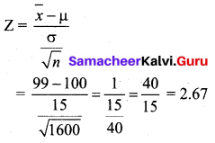
Test statistic
Samacheer Kalvi 12th Business Maths Solutions Chapter 8 Sampling Techniques and Statistical Inference Miscellaneous Problems Q7
The significant value or table value \(Z_{\alpha / 2}\) = 1.96. Comparing the values, we see that 2.67 > 1.96 (or) Z > \(Z_{\alpha / 2}\) at 5% level of significance. So the null hypothesis is rejected. Hence we conclude that the random sample is not taken from a population with mean I.Q = 100 and S.D = 15.

Samacheer Kalvi 12th Business Maths Solutions Chapter 8 Sampling Techniques and Statistical Inference Ex 8.3

Students can download 12th Business Maths Chapter 8 Sampling Techniques and Statistical Inference Ex 8.3 Questions and Answers, Samacheer Kalvi 12th Business Maths Book Solutions Guide Pdf helps you to revise the complete Tamilnadu State Board New Syllabus and score more marks in your examinations.

Tamilnadu Samacheer Kalvi 12th Business Maths Solutions Chapter 8 Sampling Techniques and Statistical Inference Ex 8.3

Choose the correct answer.

Question 1.
A ______ may be finite or infinite according to as the number of observations or items in it is finite or infinite.
(a) Population
(b) census
(c) parameter
(d) none of these
Answer:
(a) Population

Question 2.
A _______ of statistical individuals in a population is called a sample.
(a) Infinite set
(b) finite subset
(c) finite set
(d) entire set
Answer:
(b) finite subset

Samacheer Kalvi 12th Business Maths Solutions Chapter 8 Sampling Techniques and Statistical Inference Ex 8.3

Question 3.
A finite subset of statistical individuals in a population is called ________
(a) a sample
(b) a population
(c) universe
(d) census
Answer:
(a) a sample

Question 4.
Any statistical measure computed from sample data is known as _______
(a) parameter
(b) statistic
(c) infinite measure
(d) uncountable measure
Answer:
(b) statistic

Samacheer Kalvi 12th Business Maths Solutions Chapter 8 Sampling Techniques and Statistical Inference Ex 8.3

Question 5.
A ______ is one where each item in the universe has an equal chance of known opportunity of being selected.
(a) Parameter
(b) random sample
(c) statistic
(d) entire data
Answer:
(b) random sample

Question 6.
A random sample is a sample selected in such a way that every item in the population has an equal chance of being included ______
(a) Harper
(b) Fisher
(c) Karl Pearson
(d) Dr. Yates
Answer:
(a) Harper

Samacheer Kalvi 12th Business Maths Solutions Chapter 8 Sampling Techniques and Statistical Inference Ex 8.3

Question 7.
Which one of the following is probability sampling?
(a) purposive sampling
(b) judgement sampling
(c) simple random sampling
(d) Convenience sampling
Answer:
(c) simple random sampling

Question 8.
In simple random sampling from a population of units, the probability of drawing any unit at the first draw is ______
(a) \(\frac{n}{\mathrm{N}}\)
(b) \(\frac{1}{\mathrm{N}}\)
(c) \(\frac{N}{\mathrm{n}}\)
(d) 1
Answer:
(b) \(\frac{1}{\mathrm{N}}\)

Samacheer Kalvi 12th Business Maths Solutions Chapter 8 Sampling Techniques and Statistical Inference Ex 8.3

Question 9.
In _______ the heterogeneous groups are divided into homogeneous groups.
(a) Non-probability sample
(b) a simple random sample
(c) a stratified random sample
(d) systematic random sample
Answer:
(c) a stratified random sample

Question 10.
Errors in sampling are of ______
(a) Two types
(b) three types
(c) four types
(d) five types
Answer:
(a) Two types

Samacheer Kalvi 12th Business Maths Solutions Chapter 8 Sampling Techniques and Statistical Inference Ex 8.3

Question 11.
The method of obtaining the most likely value of the population parameter using statistic is called ________
(a) estimation
(b) estimator
(c) biased estimate
(d) standard error
Answer:
(a) estimation

Question 12.
An estimator is a sample statistic used to estimate a ______
(a) population parameter
(b) biased estimate
(c) sample size
(d) census
Answer:
(a) population parameter

Samacheer Kalvi 12th Business Maths Solutions Chapter 8 Sampling Techniques and Statistical Inference Ex 8.3

Question 13.
________ is a relative property, which states that one estimator is efficient relative to another.
(a) efficiency
(b) sufficiency
(c) unbiased
(d) consistency
Answer:
(a) efficiency

Question 14.
If probability P[|\(\bar{\theta}\) – θ| < ε] → 1µ as n → ∞ for any positive ε then \(\bar{\theta}\) is said to ______ estimator of θ.
(a) efficient
(b) sufficient
(c) unbiased
(d) consistent
Answer:
(d) consistent

Samacheer Kalvi 12th Business Maths Solutions Chapter 8 Sampling Techniques and Statistical Inference Ex 8.3

Question 15.
An estimator is said to be _______ if it contains all the information in the data about the
parameter it estimates.
(a) efficient
(b) sufficient
(c) unbiased
(d) consistent
Answer:
(b) sufficient

Question 16.
An estimate of a population parameter given by two numbers between which the parameter would be expected to lie is called an _______ interval estimate of the parameter.
(a) point estimate
(b) interval estimation
(c) standard error
(d) confidence
Answer:
(b) interval estimation

Samacheer Kalvi 12th Business Maths Solutions Chapter 8 Sampling Techniques and Statistical Inference Ex 8.3

Question 17.
A ________ is a statement or an assertion about the population parameter.
(a) hypothesis
(b) statistic
(c) sample
(d) census
Answer:
(a) hypothesis

Question 18.
Type I error is ______
(a) Accept H0 when it is true
(b) Accept H0 when it is false
(c) Reject H0 when it is true
(d) Reject H0 when it is false
Answer:
(c) Reject H0 when it is true

Samacheer Kalvi 12th Business Maths Solutions Chapter 8 Sampling Techniques and Statistical Inference Ex 8.3

Question 19.
Type II error is ______
(a) Accept H0 when it is wrong
(b) Accept H0 when it is true
(c) Reject H0 when it is true
(d) Reject H0 when it is false
Answer:
(a) Accept H0 when it is wrong

Question 20.
The standard error of sample mean is ________
(a) \(\frac{\sigma}{\sqrt{2 n}}\)
(b) \(\frac{\sigma}{n}\)
(c) \(\frac{\sigma}{\sqrt{n}}\)
(d) \(\frac{\sigma^{2}}{\sqrt{n}}\)
Answer:
(c) \(\frac{\sigma}{\sqrt{n}}\)

Samacheer Kalvi 12th Business Maths Solutions Chapter 7 Probability Distributions Ex 7.3

Students can download 12th Business Maths Chapter 7 Probability Distributions Ex 7.3 Questions and Answers, Samacheer Kalvi 12th Business Maths Book Solutions Guide Pdf helps you to revise the complete Tamilnadu State Board New Syllabus and score more marks in your examinations.

Tamilnadu Samacheer Kalvi 12th Business Maths Solutions Chapter 7 Probability Distributions Ex 7.3

Question 1.
Define Normal distribution.
Solution:
A random variable X is said to follow a normal distribution with parameters µ (mean) and σ2 (variance) if its probability density function is given by
Samacheer Kalvi 12th Business Maths Solutions Chapter 7 Probability Distributions Ex 7.3 Q1

Question 2.
Define Standard normal variate.
Solution:
A random variable Z = \(\frac{X-\mu}{\sigma}\) is called a standard normal variate with mean 0 and standard deviation 1 (i.e.) Z ~ N (0, 1). Its probability density function is given by
Samacheer Kalvi 12th Business Maths Solutions Chapter 7 Probability Distributions Ex 7.3 Q2

Samacheer Kalvi 12th Business Maths Solutions Chapter 7 Probability Distributions Ex 7.3

Question 3.
Write down the conditions in which the Normal distribution is a limiting case of the binomial distribution.
Solution:
The Normal distribution is a limiting case of Binomial distribution under the following conditions:

  • n, the number of trials is infinitely large, i.e. n → ∞
  • neither p (or q ) is very small.

Question 4.
Write down any five chief characteristics of Normal probability curve.
Solution:
Chief Characteristics of the Normal Probability Curve are as follows:

  • The curve is bell-shaped and symmetrical about the line x = µ.
  • Mean, median and mode of the distribution coincide.
  • The total area under the normal curve is equal to unity.
  • For a given µ and σ, there is only one normal distribution.
  • The Points of inflexion are given by x = µ ± σ

Samacheer Kalvi 12th Business Maths Solutions Chapter 7 Probability Distributions Ex 7.3

Question 5.
In a test on 2,000 electric bulbs, it was found that bulbs of a particular make, was normally distributed with an average life of 2,040 hours and a standard deviation of 60 hours. Estimate the number of bulbs likely to burn for
(i) more than 2,150 hours
(ii) less than 1,950 hours
(iii) more 1,920 hours but less than 2,100 hours.
Solution:
Let X be the numbers of hours for which the bulbs are in use. It is given that X is normally distributed with mean 2040 hours and a standard deviation of 60 hours, (i.e) X ~ N (2040, 602)
(i) P (X > 2150)
We change to the standard normal variate.
Samacheer Kalvi 12th Business Maths Solutions Chapter 7 Probability Distributions Ex 7.3 Q5
The total area to the right of Z = 0 is 0.5.
The area between Z = 0 and 1.833 is 0.4664 (from tables)
So P (Z > 1.833) = 0.5 – 0.4664 = 0.0336
The number of bulbs likely to bum for more than 2150 hours is 2000 × 0.0336 = 67.2 ~ 67

(ii) We want P (X < 1950)
= P(\(\frac{\mathrm{X}-\mu}{\sigma}<\frac{1950-2040}{60}\))
= P(Z < -1.5)
The area between Z = -1.5 and Z = 0 is same as area between Z = 0 and Z = 1.5.
From the tables, area between Z = 0 and Z = 1.5 is 0.4332
P(Z < -1.5) = 0.5 – 0.4332 = 0.0668
Hence the number of bulbs likely to bum for less than 1950 hours is 2000 × 0.0668 = 133.6 ~ 134
Samacheer Kalvi 12th Business Maths Solutions Chapter 7 Probability Distributions Ex 7.3 Q5.1

(iii) We want P(1920 < X < 2100)
When X = 1920,
\(Z=\frac{X-\mu}{\sigma}=\frac{1920-2040}{60}=-2\)
When X = 2100,
\(\mathrm{Z}=\frac{2100-2040}{60}=\frac{60}{60}=1\)
Samacheer Kalvi 12th Business Maths Solutions Chapter 7 Probability Distributions Ex 7.3 Q5.2
So P(1920 < X < 2100) = P(-2 < Z < 1)
= P(-2 < Z < 0) + P(0 < Z < 1)
= P (0 < Z < 2) + P (0 < Z < 1)
= 0.4772 + 0.3413
= 0.8185
Hence the number of bulbs likely to bum for more than 1920 hours but less than 2100 hours is 2000 × 0.8185 = 1637.

Samacheer Kalvi 12th Business Maths Solutions Chapter 7 Probability Distributions Ex 7.3

Question 6.
In a distribution, 30% of the items are under 50 and 10% are over 86. Find the mean and standard deviation of the distribution.
Solution:
Let X be the normal random variable denoting the number of items in the distribution.
It is given that 30% of items are under 50
⇒ P (X < 50) = 30% = 0.3.
Also, 10% are over 86
⇒ P (X > 86) = 10% = 0.1.
We have to find µ and σ.
Representing the given data diagrammatically,
Where Z1 = \(\frac{50-\mu}{\sigma}\) and Z2 = \(\frac{86-\mu}{\sigma}\)
Samacheer Kalvi 12th Business Maths Solutions Chapter 7 Probability Distributions Ex 7.3 Q6
From the diagram,
P (-Z1 < Z < 0) = 0.2
By symmetry P (0 < Z < Z1) = 0.2
Z1 = 0.525 (from the normal table)
Hence -0.525 = \(\frac{50-\mu}{\sigma}\)
(i.e.) 50 – µ = -0.525σ …….. (1)
Again P(0 < Z < Z2) = 0.4
Z2 = 1.28
Hence \(\frac{86-\mu}{\sigma}\) = 1.28
(or) 86 – µ = 1.28σ ……. (2)
Solving (1) and (2)
50 – µ = -0.525σ
86 – µ = 1.28σ
Subtracting,
36 = 1.28σ + 0.525σ
36 = 1.805σ
σ = 19.94
Using this in (2),
86 – µ = 1.28 (19.94)
86 – µ = 25.52
µ = 60.48
Hence the mean of the distribution is 60.48 and standard deviation is 19.94.

Question 7.
X is normally distributed with mean 12 and SD 4. Find P(X ≤ 20) and P(0 ≤ X ≤ 12).
Solution:
Given X ~ N (12, 42), (i.e) mean (µ) = 12 and s.d (σ) = 4.
P(X ≤ 20)
= P(\(\frac{X-\mu}{\sigma} \leq \frac{20-12}{4}\))
= P(X ≤ 2)
Now P(Z ≤ 2) = P(Z ≤ 0) + P(0 ≤ Z ≤ 2)
= 0.5 + 0.4772
= 0.9772
Samacheer Kalvi 12th Business Maths Solutions Chapter 7 Probability Distributions Ex 7.3 Q7

Samacheer Kalvi 12th Business Maths Solutions Chapter 7 Probability Distributions Ex 7.3

P(0 ≤ X ≤ 12)
= P(\(\frac{0-12}{4} \leq \frac{X-\mu}{\sigma} \leq \frac{12-12}{4}\))
= P (-3 ≤ Z ≤ 0)
= P(0 ≤ Z ≤ 3)
P(0 ≤ Z ≤ 3) = 0.49865 (from normal tables)
Samacheer Kalvi 12th Business Maths Solutions Chapter 7 Probability Distributions Ex 7.3 Q7.1

Question 8.
If the heights of 500 students are normally distributed with mean 68.0 inches and standard deviation of 3.0 inches, how many students have height
(a) greater than 72 inches
(b) less than or equal to 64 inches
(c) between 65 and 71 inches.
Solution:
Given X is the normal random variables denoting the height of the students with mean µ = 68 and s.d (σ) = 3.
(a) To find P(X > 72)
= P(Z > \(\frac{72-68}{3}\))
= P(Z > \(\frac{4}{3}\))
= P(Z > 1.33)
Now P(Z > 1.33) = 0.5 – P(0 < Z < 1.33)
= 0.5 – 0.4082
= 0.0918
Hence number of students whose height is greater than 72 inches is 500 × 0.0918 = 45.9 ~ 46
Samacheer Kalvi 12th Business Maths Solutions Chapter 7 Probability Distributions Ex 7.3 Q8

(b) To find P(X ≤ 64)
= P(Z ≤ \(\frac{64-68}{3}\))
= P(Z ≤ -1.33)
By Symmetry,
P(Z ≤ -1.33) = P(Z ≥ 1.33) = 0.0918 (see before section)
Hence number of students whose heights are less than or equal to 64 inches is 0.0918 × 500 = 46
Samacheer Kalvi 12th Business Maths Solutions Chapter 7 Probability Distributions Ex 7.3 Q8.1

(c) To find P (65 < X < 71)
= P(\(\frac{65-68}{3}\) < Z < \(\frac{71-68}{3}\))
= P(-1 < Z < 1)
= P(-1 < Z < 0) + P(0 < Z < 1)
= 2P(0 < Z < 1) {By symmetry}
= 2 (0.3413)
= 0.6826
Hence number of students with height between 65 and 71 inches is (500) (0.6826) = 341.3 ~ 342.
Samacheer Kalvi 12th Business Maths Solutions Chapter 7 Probability Distributions Ex 7.3 Q8.2

Question 9.
In a photographic process, the developing time of prints may be looked upon as a random variable having the normal distribution with a mean of 16.28 seconds and a standard deviation of 0.12 second. Find the probability that it will take less than 16.35 seconds to develop prints.
Solution:
Let X be the normal random variable denoting the developing time of the prints.
Given that mean µ = 16.28 and s.d σ = 0.12
To find P(X < 16.35)
When X = 16.35, \(\mathrm{Z}=\frac{\mathrm{X}-\mu}{\sigma}=\frac{16.35-16.28}{0.12}\)
Z = 0.58
So P(X < 16.35) = P(Z < 0.58)
Now P(Z < 0.58) = 0.5 + P(0 < Z < 0.58)
= 0.5 + 0.2190
= 0.7190
Thus the probability that it will take less than 16.35 seconds to develop prints is 0.719.
Samacheer Kalvi 12th Business Maths Solutions Chapter 7 Probability Distributions Ex 7.3 Q9

Samacheer Kalvi 12th Business Maths Solutions Chapter 7 Probability Distributions Ex 7.3

Question 10.
Time taken by a construction company to construct a flyover is a normal variate with mean 400 labour days and a standard deviation of 100 labour days. If the company promises to construct the flyover in 450 days or less and agree to pay a penalty of ₹ 10,000 for each labour day spent in excess of 450. What is the probability that
(i) the company pays a penalty of at least ₹ 2,00,000?
(ii) the company takes at most 500 days to complete the flyover?
Solution:
Let X be the normal variate denoting the number of labour days.
Given mean µ = 400 and s.d σ = 100
(i) The company pays penalty of ₹ 2,00,000 at the rate of ₹ 10,000 per each extra labour day.
No. of extra days = \(\frac{2,00,000}{10,000}\) = 20
So the probability that company pays a penalty of atleast ₹ 2,00,000 is probability that labour days should be atleast 450 + 20 = 470 days, (i.e.) P (X ≥ 470)
Now P(X ≥ 470) = P(Z ≥ \(\frac{470-400}{100}\)) = P (Z ≥ 0.7)
P(Z ≥ 0.7) = 0.5 – P(0 ≤ Z ≤ 0.7) = 0.5 – 0.258 = 0.242
Samacheer Kalvi 12th Business Maths Solutions Chapter 7 Probability Distributions Ex 7.3 Q10

(ii) P (X ≤ 500) = P(Z ≤ \(\frac{500-40}{100}\)) = P (Z ≤ 1)
P(Z ≤ 1) = 0.5 + P (0 ≤ Z ≤ 1) = 0.5 + 0.3413 = 0.8413
Thus the probability that the company takes at most 500 days to complete the flyover is 0.8413.
Samacheer Kalvi 12th Business Maths Solutions Chapter 7 Probability Distributions Ex 7.3 Q10.1

Samacheer Kalvi 12th Business Maths Solutions Chapter 8 Sampling Techniques and Statistical Inference Ex 8.2

Students can download 12th Business Maths Chapter 8 Sampling Techniques and Statistical Inference Ex 8.2 Questions and Answers, Samacheer Kalvi 12th Business Maths Book Solutions Guide Pdf helps you to revise the complete Tamilnadu State Board New Syllabus and score more marks in your examinations.

Tamilnadu Samacheer Kalvi 12th Business Maths Solutions Chapter 8 Sampling Techniques and Statistical Inference Ex 8.2

Question 1.
Mention two branches of statistical inference?
Solution:
The two branches of statistical inference are estimation and testing of hypothesis.

Question 2.
What is an estimator?
Answer:
An estimator is a statistic that is used to infer the value of an unknown population parameter in a statistical model. The estimator is a function of the data arid so it is also a random variable.

Samacheer Kalvi 12th Business Maths Solutions Chapter 8 Sampling Techniques and Statistical Inference Ex 8.2

Question 3.
What is an estimate?
Solution:
Any specific numerical value of the estimator is called an estimate. For example, sample means are used to estimate population means.

Question 4.
What is point estimation?
Solution:
Point estimation involves the use of sample data to calculate a single value which is to serve as a best estimate of an unknown population parameter. For example the mean height of 145 cm from a sample of 15 students is‘a point estimate for the mean height of the class of 100 students.

Samacheer Kalvi 12th Business Maths Solutions Chapter 8 Sampling Techniques and Statistical Inference Ex 8.2

Question 5.
What is interval estimation?
Solution:
Interval estimation is the use of sample data to calculate an interval of possible values of an unknown population parameter. For example the interval estimate for the population mean is (101.01, 102.63).This gives a range within which the population mean is most likely to be located.

Question 6.
What is confidence interval?
Solution:
A confidence interval L a type of interval estimate, computed from the statistics of the observed data, that might contain the true value of an unknown population parameter. The numbers at the upper and lower end of a confidence interval are called confidence limits. For example, if mean is 7.4 with confidence interval (5.4, 9.4), then the numbers 5.4 and 9.4 are the confidence limits.

Question 7.
What is null hypothesis? Give an example.
Solution:
A null hypothesis is a type of hypothesis, that proposes that no statistical significance exists in a set of given observations. For example, let the average time to cook a specific dish is 15 minutes. The null hypothesis would be stated as “The population mean is equal to 15 minutes”, (i.e) H0 : µ = 15

Samacheer Kalvi 12th Business Maths Solutions Chapter 8 Sampling Techniques and Statistical Inference Ex 8.2

Question 8.
Define the alternative hypothesis.
Solution:
The alternative hypothesis is the hypothesis that is contrary to the null hypothesis and it is denoted by H1.
For example if H1 : µ = 15, then the alternative hypothesis will be : H1 : µ ≠ 15, (or) H1 : µ < 15 (or) H1 : µ > 15.

Question 9.
Define the critical region.
Solution:
The critical region is the region of values that corresponds to the rejection of the null hypothesis at some chosen probability level. For the two-tailed test, the critical region is given below.
Samacheer Kalvi 12th Business Maths Solutions Chapter 8 Sampling Techniques and Statistical Inference Ex 8.2 Q9
where α is the level of significance.

Question 10.
Define critical value.
Solution:
A critical value is a point on the test distribution that is compared to the test statistic to determine whether to reject the null hypothesis. It depends on the level of significance. For example, if the confidence level is 90% then the critical value is 1.645.

Question 11.
Define the level of significance
Solution:
The level of significance is defined as the probability of rejecting a null hypothesis by the test when it is really true, which is denoted as α. That is P(Type 1 error) = α. For example, the level of significance 0.1 is related to the 90% confidence level.

Samacheer Kalvi 12th Business Maths Solutions Chapter 8 Sampling Techniques and Statistical Inference Ex 8.2

Question 12.
What is a type I error?
Solution:
In statistical hypothesis testing, a Type f error is the rejection of a true null hypothesis. Example of Type I errors includes a test that shows a patient to have a disease when he does not have the disease, a fire alarm going on indicating a fire when there is no fire (or) an experiment indicating that medical treatment should cure a disease when in fact it does not.

Question 13.
What is the single-tailed test?
Solution:
A single-tailed test or a one-tailed test is a statistical test in which the critical area of a distribution is one-sided so that it is either greater than or less than a certain value, but not both. For the null hypothesis H0 : µ = 16.91, the alternative hypothesis H1 : µ > 16.91 or H1 : µ < 16.91 are one-tailed tests.

Question 14.
A sample of 100 items, draw from a universe with mean value 4 and S.D 3, has a mean value 3.5. Is the difference in the mean significant?
Solution:
Given Sample size n = 100
Sample mean \(\bar{x}\) = 3.5
Population mean µ = 4
Population SD σ = 3
Now, null hypothesis H0 : µ = 4
Alternative hypothesis H1 : µ ≠ 4 (Two tail)
We take level of significance α = 5% = 0.05
The table value \(\mathrm{Z}_{\alpha / 2}\) = 1.96
Test statistic
Samacheer Kalvi 12th Business Maths Solutions Chapter 8 Sampling Techniques and Statistical Inference Ex 8.2 Q14
Since the alternative hypothesis is of the two-tailed test we can take |Z| = 1.667. We observe that 1.667 < 1.96 (i.e) |Z| < \(\mathrm{Z}_{\alpha / 2}\). So at 5% level of significance, the null hypothesis H0 is accepted. Therefore, we conclude that there is no significant difference between the sample mean and the population mean.

Samacheer Kalvi 12th Business Maths Solutions Chapter 8 Sampling Techniques and Statistical Inference Ex 8.2

Question 15.
A sample of 400 individuals is found to have a mean height of 67.47 inches. Can it be reasonably regarded as a sample from a large population with a mean height of 67.39 inches and standard deviation of 1.30 inches?
Solution:
Given Sample size n = 400
Sample mean \(\bar{x}\) = 67.47
Population mean µ = 67.39
Population SD σ = 1.3
Null hypothesis H0 : µ = 67.39 inches
(the sample has been drawn from the population with mean heights 67.39 inches)
Alternative hypothesis H1 : µ ≠ 67.39 inches
(the sample has not been drawn from the population with mean height 67.39 inches)
The level of significance α = 5% = 0.05
Test statistic
Samacheer Kalvi 12th Business Maths Solutions Chapter 8 Sampling Techniques and Statistical Inference Ex 8.2 Q15
The significant value or table value \(\mathrm{Z}_{\alpha / 2}\) = 1.96. We see that 1.2308 < 1.96 (i.e) Z < \(\mathrm{Z}_{\alpha / 2}\). Since the calculated value is less than the table value at 5% level of significance, the null hypothesis is accepted. Hence we conclude that the data does not provide us with any evidence against the null hypothesis. Thus, the sample has been drawn from a large population with a mean height of 67.39 inches and S.D 1.3 inches.

Question 16.
The average score on a nationally administered aptitude test was 76 and the corresponding standard deviation was 8. In order to evaluate a state’s education system, the scores of 100 of the state’s students were randomly selected. These students had an average score of 72. Test at a significance level of 0.05 if there is a significant difference between the state scores and the national scores.
Solution:
Given Population mean µ = 76
Population SD σ = 8
Sample size n = 100
Sample mean \(\bar{x}\) = 72
Significance level α = 0.05
Null hypothesis H0 : µ = 76
(i.e) there is no difference between the state scores and the national scores.
Alternative hypothesis H1 : µ ≠ 76
(i.e) there is a significant difference between the state scores and the nationals scores of the aptitude test.
Test statistic
Samacheer Kalvi 12th Business Maths Solutions Chapter 8 Sampling Techniques and Statistical Inference Ex 8.2 Q16
The significant value or table value \(\mathrm{Z}_{\alpha / 2}\) = 1.96. Comparing the calculated value and table value, we find that |Z| > \(\mathrm{Z}_{\alpha / 2}\) (i.e) 5 > 1.96. So the null hypothesis is rejected and we accept the alternative hypothesis. So we conclude that at the significance level of 5%, there is a difference between the state scores and the national scores of the nationally administered amplitude test.

Samacheer Kalvi 12th Business Maths Solutions Chapter 8 Sampling Techniques and Statistical Inference Ex 8.2

Question 17.
The mean breaking strength of cables supplied by a manufacturer is 1,800 with a standard deviation of 100. By a new technique in the manufacturing process it is claimed that the breaking strength of the cables has increased. In order to test this claim a sample of 50 cables is tested. It is found that the mean breaking strength is 1,850. Can you support the claim at 0.01 level of significance?
Solution:
Given Population mean µ = 1800
Population SD σ = 100
Sample size n = 50
Sample mean \(\bar{x}\) = 1850
Significance level α = 0.01
Null hypothesis H0 : µ = 1800
(i.e) the breaking strength of the cables has not increased, after the new technique in the manufacturing process.
Alternative hypothesis H1 : µ > 1800 (i.e) the new technique was successful.
Test statistic
Samacheer Kalvi 12th Business Maths Solutions Chapter 8 Sampling Techniques and Statistical Inference Ex 8.2 Q17
The table value for the one-tailed test is Zα = 2.33.
Comparing the calculated value and table value, we find that Z > Zα (i.e.) 3.536 > 2.33.

Inference: Since the calculated value is greater than the table value at 1 % level of significance, the null hypothesis is rejected and we accept the alternative hypothesis. We conclude that by the new technique in the manufacturing process the breaking strength of the cables is increased. So the claim is supported at 0.01 level of significance.

Samacheer Kalvi 12th Business Maths Solutions Chapter 7 Probability Distributions Ex 7.2

Students can download 12th Business Maths Chapter 7 Probability Distributions Ex 7.2 Questions and Answers, Samacheer Kalvi 12th Business Maths Book Solutions Guide Pdf helps you to revise the complete Tamilnadu State Board New Syllabus and score more marks in your examinations.

Tamilnadu Samacheer Kalvi 12th Business Maths Solutions Chapter 7 Probability Distributions Ex 7.2

Question 1.
Define Poisson distribution.
Solution:
Poisson distribution is a discrete frequency distribution which gives the probability of a number of independent events occurring in a fixed time. It is useful for characterizing events with very low probabilities of occurrence within some definite time or space.

Question 2.
Write any 2 examples for Poisson distribution.
Solution:
Examples of Poisson distribution are given by

  • The number of printing mistakes per page in a textbook.
  • A number of lightning per second.
  • The number of bacteria in one cubic centimetre.

Samacheer Kalvi 12th Business Maths Solutions Chapter 7 Probability Distributions Ex 7.2

Question 3.
Write the conditions for which the Poisson distribution is a limiting case of the binomial distribution.
Solution:
Poisson distribution is a limiting case of binomial distribution under the following conditions:

  • the number of trials ‘n’ is indefinitely large i.e, → ∞
  • the probability of success ‘p’ in each trial is very small, i.e, p → 0
  • np = λ is finite. Thus p = \(\frac{\lambda}{n}\) and q = 1 – \(\frac{\lambda}{n}\), λ > 0

Question 4.
Derive the mean and variance of the Poisson distribution.
Solution:
Let X be a Poisson random variable with parameter λ. The p.m.f is given by
Samacheer Kalvi 12th Business Maths Solutions Chapter 7 Probability Distributions Ex 7.2 Q4
Samacheer Kalvi 12th Business Maths Solutions Chapter 7 Probability Distributions Ex 7.2 Q4.1
Samacheer Kalvi 12th Business Maths Solutions Chapter 7 Probability Distributions Ex 7.2 Q4.2
Thus the mean and variance of Poisson distribution are both equal to λ.

Samacheer Kalvi 12th Business Maths Solutions Chapter 7 Probability Distributions Ex 7.2

Question 5.
Mention the properties of Poisson distribution.
Solution:

  1. Poisson distribution is the only distribution in which the mean and variance are equal.
  2. The probability that an event occurs in a given time, distance, area or volume is the same.

Question 6.
The mortality rate for a certain disease is 7 in 1000. What is the probability for just 2 deaths on account of this disease in a group of 400? [Given e-2.8 = 0.06]
Solution:
Let X denote the number of deaths due to the disease
P(death) = \(\frac{7}{1000}\) = 0.007 ⇒ p = 0.007 and n = 400
The value of mean λ = np = (0.007) (400) = 2.8
Hence X follows a Poisson distribution with
Samacheer Kalvi 12th Business Maths Solutions Chapter 7 Probability Distributions Ex 7.2 Q6
So the probability of just 2 deaths on account of this disease in a group of 400 is 0.2352.

Samacheer Kalvi 12th Business Maths Solutions Chapter 7 Probability Distributions Ex 7.2

Question 7.
It is given that 5% of the electric bulbs manufactured by a company are defective. Using Poisson distribution find the probability that a sample of 120 bulbs will contain no defective bulb.
Solution:
Given p = \(\frac{5}{100}\) = 0.05 and n = 120
⇒ λ = np = (0.05) (120) = 6
Thus X is a Poisson random variable with P (X = x) = \(\frac{e^{-6} 6^{x}}{x !}\)
We want P (no defective bulb) = P (X = 0)
= \(\frac{e^{-6} 6^{0}}{0 !}\)
= e-6
= 0.0025 (Using exponent table)
Thus the probability that a sample of 120 bulbs will not contain any defective bulb is 0.0025.

Question 8.
A car hiring firm has two cars. The demand for cars on each day is distributed as a Poisson variate, with mean 1.5. Calculate the proportion of days on which
(i) Neither car is used
(ii) Some demand is refused.
Solution:
Let X be the Poisson variable denoting the demand for the cars.
It is given that mean is 1.5 ⇒ λ = 1.5
(i) P (Neither car is used) = P (X = 0) = \(\frac{e^{-1.5}(1.5)^{0}}{0 !}=e^{-1.5}=0.2231\)
(ii) Some demand is refused when demand is more than 2 since the firm has only 2 cars. So we want P (X > 2)
Now P (X > 2) = 1 – P (X ≤ 2)
= 1 – [P(X = 2) + P(X = 1) + P(X = 0)]
Samacheer Kalvi 12th Business Maths Solutions Chapter 7 Probability Distributions Ex 7.2 Q8

Samacheer Kalvi 12th Business Maths Solutions Chapter 7 Probability Distributions Ex 7.2

Question 9.
The average number of phone calls per minute into the switchboard of a company between 10.00 am and 2.30 pm is 2.5. Find the probability that during one particular minute there will be
(i) no phone at all
(ii) exactly 3 calls
(iii) at least 5 calls.
Solution:
Let X be the Poisson variable denoting the number of phone calls per minute.
Samacheer Kalvi 12th Business Maths Solutions Chapter 7 Probability Distributions Ex 7.2 Q9
P (X = 1) = \(\frac{e^{-2.5}(2.5)}{1 !}\) = (0.08208) (2.5) = 0.2052
Using the above values and P (X = 0) and P (X = 3) from the previous subdivisions in (A) we get,
P(X ≥ 5) = 1 – [0.1336 + 0.2138 + 0.2565 + 0.2052 + 0.08208]
= 1 – 0.89118
= 0.10882

Question 10.
The distribution of the number of road accidents per day in a city is Poisson with mean 4. Find the number of days out of 100 days when there will be
(i) no accident
(ii) at least 2 accidents and
(iii) at most 3 accidents.
Solution:
Let X be the Poisson variable denoting the number of accidents per day.
Given that mean is 4 (i.e,) λ = 4. The p.m.f is given by P(X = x) = \(\frac{e^{-4} 4^{x}}{x !}\)
(i) P (no accident) = P(X = 0) = e-4 = 0.0183
For 100 days we have 100 × 0.0183 = 1.83 ~ 2
Hence out of 100 days there will be no accident for 2 days.

(ii) P (atleast 2 accidents) = P (X ≥ 2)
= 1 – P (X < 2)
= 1 – [P(X = 1) + P(X = 0)]
= 1 – [e-4 (4) + e-4]
= 1 – (0.0183) (5)
= 1 – 0.0915
= 0.9085
For 100 days we have 100 × 0.9085 ~ 91
Hence out of 100 days there will be at least 2 accidents for 91 days.

(iii) P (atmost 3 accidents) = P (X ≤ 3)
= P (X = 0 ) + P (X = 1 ) + P (X = 2) + P (X = 3)
= \(e^{-4}\left[1+\frac{4}{1}+\frac{16}{2}+\frac{64}{6}\right]\)
= (0.0183) [23.6667]
= 0.4331
For 100 days we have 100 × 0.4331 ~ 43
Hence out of 100 days, there will be atmost 3 accidents for 43 days.

Samacheer Kalvi 12th Business Maths Solutions Chapter 7 Probability Distributions Ex 7.2

Question 11.
Assuming that a fatal accident in a factory during the year is 1/1200, calculate the probability that in a factory employing 300 workers there will be at least two fatal accidents in a year, (given e-0.25 = 0.7788).
Solution:
Let X denote the number of accidents.
Given that probability of accidents ‘p’ is 1/1200 and n = 300
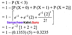
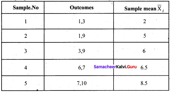
Samacheer Kalvi 12th Business Maths Solutions Chapter 7 Probability Distributions Ex 7.2 Q11
= 1 – [e-0.25 + e-0.25 (0.25)]
= 1 – e-0.25 (1.25)
= 1 – (0.7788) (1.25)
= 0.0265
Thus the probability that there will be atleast two fatal accidents in a year is 0.0265.

Question 12.
The average number of customers, who appear in a counter of a certain bank per minute is two. Find the probability that during a given minute
(i) No customer appears
(ii) three or more customers appear.
Solution:
Let X denote the number of customers.
Given λ = 2
(i) P (no customer) = P (X = 0)
= \(\frac{e^{-2}(2)^{0}}{0 !}\)
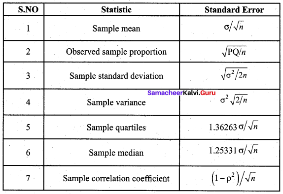
= e-2
= 0.1353
(ii) P (3 or more customers) = P (X ≥ 3)
Samacheer Kalvi 12th Business Maths Solutions Chapter 7 Probability Distributions Ex 7.2 Q12
Thus during a given minute, the probability that three or more customers appear is 0.3235.

Samacheer Kalvi 12th Business Maths Solutions Chapter 8 Sampling Techniques and Statistical Inference Ex 8.1

Students can download 12th Business Maths Chapter 8 Sampling Techniques and Statistical Inference Ex 8.1 Questions and Answers, Samacheer Kalvi 12th Business Maths Book Solutions Guide Pdf helps you to revise the complete Tamilnadu State Board New Syllabus and score more marks in your examinations.

Tamilnadu Samacheer Kalvi 12th Business Maths Solutions Chapter 8 Sampling Techniques and Statistical Inference Ex 8.1

Question 1.
What is the population?
Solution:
A population is a set of similar items or events which is of interest for some question or experiment. A population can be specific or vague. Examples of population defined vaguely include the number of newborn babies in Tamil Nadu, a total number of tech startups in India, the average height of all exam candidates, mean weight of taxpayers in Chennai etc. Examples of population defined specifically include a number of fans produced in a particular factory, the number of students in a class, the number of boys and girls in a tuition centre etc.

Question 2.
What is the sample?
Solution:
A sample is a set of data collected from a statistical population by a defined procedure. The elements of a sample are called sample size or sample points. Samples are collected and statistics are calculated from the samples, so that one can make inferences from the sample to the population.

Samacheer Kalvi 12th Business Maths Solutions Chapter 8 Sampling Techniques and Statistical Inference Ex 8.1

Question 3.
What is statistic?
Solution:
A statistic is used to estimate the value of a population parameter. For instance, we selected a random sample of 100 students from a school with 1000 students. The average height of the sampled students would be an example of a statistic. Examples, sample variance, sample quartiles, sample percentiles, sample moments etc.

Question 4.
Define parameter.
Solution:
A parameter is any numerical quantity that characterizes a given population or some aspect of it. This means the parameter tells us something about the whole population. For example, the population mean µ, variance σ2, population proportion P, population correlation ρ.

Samacheer Kalvi 12th Business Maths Solutions Chapter 8 Sampling Techniques and Statistical Inference Ex 8.1

Question 5.
What is the sampling distribution of a statistic?
Solution:
Sampling distribution of a statistic is the probability distribution of a given random sample based statistic. It may be considered as the distribution of the statistic for all possible samples from the same population of a given sample size.
Example, the sampling distribution of the mean for n = 2 is given below:
Samacheer Kalvi 12th Business Maths Solutions Chapter 8 Sampling Techniques and Statistical Inference Ex 8.1 Q5

Question 6.
What is the standard error?
Solution:
The standard error (S.E) of a statistic is the standard deviation of its sampling distribution. If the parameter or the statistic is the mean, it is called the standard error of the mean (SEM). The standard error provides a rough estimate of the interval in which the population parameters is likely to fall.
Samacheer Kalvi 12th Business Maths Solutions Chapter 8 Sampling Techniques and Statistical Inference Ex 8.1 Q6

Samacheer Kalvi 12th Business Maths Solutions Chapter 8 Sampling Techniques and Statistical Inference Ex 8.1

Question 7.
Explain in detail about simple random sampling with a suitable example.
Solution:
(i) Simple random sampling:
In this technique, the samples are selected in such a way that each and every unit in the population has an equal and independent chance of being selected as a sample. Simple random sampling may be done, with or without replacement of the samples selected. In a simple random sampling with replacement, there is a possibility of selecting the same sample any number of times. So, simple random sampling without replacement is followed.
Thus in simple random sampling from a population of N units, the probability of drawing any unit at the first draw is \(\frac{1}{N}\), the probability of drawing any unit in the second draw from among the available (N – 1) units is \(\frac{1}{(N-1)}\), and so on. Several methods have been adopted for random selection of the samples from the population. Of those, the following two methods are generally used and which are described below.

1. Lottery method
This is the most popular and simplest method when the population is finite. In this method, all the items of the population are numbered on separate slips of paper of the same size, shape and colour. They are folded and placed in a container and shuffled thoroughly. Then the required numbers of slips are selected for the desired sample size. The selection of items thus depends on chance.

For example, if we want to select 10 students, out of 100 students, then we must write the names/roll number of all the 100 students on slips of the same size and mix them, then we make a blindfold selection of 10 students. This method is called unrestricted random sampling because units are selected from the population without any restriction. This method is mostly used in lottery draws. If the population or universe is infinite, this method is inapplicable.

2. Table of Random number
When the population size is large, it is difficult to number all the items on separate slips of paper of same size, shape and colour. The alternative method is that of using the table of random numbers. The most practical, easy and inexpensive method of selecting a random sample can be done through “Random Number Table”. The random number table has been so constructed that each of the digits 0, 1, 2,…, 9 will appear approximately with the same frequency and independently of each other.

The various random number tables available are

  • L.H.C. Tippett random number series
  • Fisher and Yates random number series
  • Kendall and Smith random number series
  • Rand Corporation random number series.

Tippett’s table of random numbers is most popularly used in practice.

An example to illustrate how Tippett’s table of random numbers may be used is given below. Suppose we have to select 20 items out of 6,000. The procedure is to number all the 6,000 items from 1 to 6,000. A page from Tippett’s table may be selected and the first twenty numbers ranging from 1 to 6,000 are noted down. If the numbers are above 6000, choose the next number ranging from 1 to 6000. Items bearing those numbers will be selected as samples from the population. Making use of the portion of the random number table given, the required random samples are shaded. Here, we consider row-wise selection of random numbers.
Samacheer Kalvi 12th Business Maths Solutions Chapter 8 Sampling Techniques and Statistical Inference Ex 8.1 Q7

Question 8.
Explain the stratified random sampling with a suitable example.
Solution:
Stratified Random Sampling
In stratified random sampling, first divide the population into subpopulations, which are called strata. Then, the samples are selected from each of the strata through random techniques. The collection of all the samples from all strata gives the stratified random samples.

When the population is heterogeneous or different segments or groups with respect to the variable or characteristic under study, then the Stratified Random Sampling method is studied.. First, the population is divided into the homogeneous number of sub-groups or strata before the sample is drawn. A sample is drawn from each stratum at random. Following steps are involved in selecting a random sample in a stratified random sampling method.

Samacheer Kalvi 12th Business Maths Solutions Chapter 8 Sampling Techniques and Statistical Inference Ex 8.1

(a) The population is divided into different classes so that each stratum will consist of more or less homogeneous elements. The strata are so designed that they do not overlap each other.
(b) After the population is stratified, a sample of a specified size is drawn at random from each stratum using Lottery Method or Table of Random Number Method.

Stratified random sampling is applied in the field of the different legislative areas as strata in election polling, division of districts (strata) in a state etc…

Ex: From the following data, select 68 random samples from the population of the heterogeneous group with a size of 500 through stratified random sampling, considering the following categories as strata.

  • Category 1: Lower income class – 39%
  • Category 2: Middle income class – 38%
  • Category 3: Upper income class – 23%

Solution:
Samacheer Kalvi 12th Business Maths Solutions Chapter 8 Sampling Techniques and Statistical Inference Ex 8.1 Q8

Question 9.
Explain in detail about systematic random sampling with example.
Solution:
Systematic sampling:
In systematic sampling, randomly select the first sample from the first k units. Then every kth member, starting with the first selected sample, is included in the sample.

Systematic sampling is a commonly used technique if the complete and up-to-date list of the sampling units is available. We can arrange the items in numerical, alphabetical, geographical or in any other order. The procedure of selecting the samples starts with selecting the first sample at random, the rest being automatically selected according to some pre-determined ( pattern. A systematic sample is formed by selecting every item from the population, where k refers to the sample interval. The sampling interval can be determined by dividing the size of the population by the size of the sample to be chosen.
That is k = \(\frac{\mathrm{N}}{n}\), where k is an integer.
k = Sampling interval, N = Size of the population, n = Sample size.

Procedure for selection of samples by systematic sampling method
(i) If we want to select a sample of 10 students from a class of 100 students, the sampling interval is calculated as \(k=\frac{N}{n}=\frac{100}{10}=10\)
Thus sampling interval = 10 denotes that for every 10 samples one sample has to be selected.
(ii) The first sample is selected from the first 10 (sampling interval) samples through random selection procedures.
(iii) If the selected first random sample is 5, then the rest of the samples are automatically selected by incrementing the value of the sampling interval (k = 10) i.e., 5, 15, 25, 35, 45, 55, 65, 75, 85, 95.

Samacheer Kalvi 12th Business Maths Solutions Chapter 8 Sampling Techniques and Statistical Inference Ex 8.1

Ex: Suppose we have to select 20 items out of 6,000. The procedure is to number all the 6,000 items from 1 to 6,000. The sampling interval is calculated as k = \(\frac{N}{n}=\frac{6000}{20}\) = 300. Thus sampling interval = 300 denotes that for every 300 samples one sample has to be selected. The first sample is selected from the first 300 (sampling interval) samples through random selection procedures. If the selected first random sample is 50, then the rest of the samples are automatically selected by incrementing the value of the sampling interval (k = 300) ie,50, 350, 650, 950, 1250, 1550, 1850, 2150, 2450, 2750, 3050, 3350, 3650, 3950, 4250, 4550, 4850, 5150, 5450, 5750. Items bearing those numbers will be selected as samples from the population.

Question 10.
Explain in detail about sampling error.
Solution:
Sampling Errors: Errors, which arise in the normal course of investigation or enumeration on account of chance, are called sampling errors. Sampling errors are inherent in the method of sampling. They may arise accidentally without any bias or prejudice.

Sampling Errors arise primarily due to the following reasons:

  • Faulty selection of the sample instead of the correct sample by defective sampling technique.
  • The investigator substitutes a convenient sample if the original sample is not available while investigation.
  • In area surveys, while dealing with borderlines it depends upon the investigator whether to include them in the sample or not. This is known as Faulty demarcation of sampling units.

Question 11.
Explain in detail about the non-sampling error.
Solution:
Non-Sampling Errors:
The errors that arise due to human factors which always vary from one investigator to another in selecting, estimating or using measuring instruments( tape, scale) are called Non-Sampling errors.
It may arise in the following ways:

  • Due to negligence and carelessness of the part of either investigator or respondents.
  • Due to the lack of trained and qualified investigators.
  • Due to the framing of a wrong questionnaire.
  • Due to applying the wrong statistical measure
  • Due to incomplete investigation and sample survey.

Question 12.
State any two merits of simple random sampling.
Solution:

  • In simple random sampling personal bias is completely eliminated.
  • This method is economical as it saves time, money and labour.

Question 13.
State any three merits of stratified random sampling.
Solution:

  • A random stratified sample is superior to a simple random sample because it ensures representation of all groups and thus it is more representative of the population which is being sampled.
  • A stratified random sample can be kept small in size without losing its accuracy.
  • It is easy to administer if the population under study is sub-divided.

Samacheer Kalvi 12th Business Maths Solutions Chapter 8 Sampling Techniques and Statistical Inference Ex 8.1

Question 14.
State any two demerits of systematic random sampling.
Solution:

  • Systematic samples are not random samples.
  • If N is not a multiple of n, then the sampling interval (k) cannot be an integer, thus sample selection becomes difficult.

Question 15.
State any two merits for systematic random sampling.
Solution:
Merits of systematic sampling are given below:

  • This method distributes the sample more evenly over the entire listed population.
  • The time and work are reduced much.

Question 16.
Using the following Tippet’s random number table.
Samacheer Kalvi 12th Business Maths Solutions Chapter 8 Sampling Techniques and Statistical Inference Ex 8.1 Q16
Draw a sample of 10 three-digit numbers which are even numbers.
Solution:
There are many ways to select a sample of 10 3-digit even numbers. From the table, start from the first number and move along the column. Select the first three digits as the number. If it is an odd number, move to the next number. The selected sample is 416, 664, 952, 748, 524, 914, 154, 340, 140, 276.
Samacheer Kalvi 12th Business Maths Solutions Chapter 8 Sampling Techniques and Statistical Inference Ex 8.1 Q16.1

Question 17.
A wholesaler in apples claims that only 4 % of the apples supplied by him are defective. A random sample of 600 apples contained 36 defective apples. Calculate the standard error concerning good apples.
Solution:
Sample size = 600
No. of defective apples = 36
Sample proportion p = \(\frac{36}{600}\) = 0.06
Population proportion P = probability of defective apples = 4% = 0.04
Q = 1 – P = 1 – 0.04 = 0.96
The S.E for sample proportion is given by S.E
Samacheer Kalvi 12th Business Maths Solutions Chapter 8 Sampling Techniques and Statistical Inference Ex 8.1 Q17

Samacheer Kalvi 12th Business Maths Solutions Chapter 8 Sampling Techniques and Statistical Inference Ex 8.1

Question 18.
A sample of 1000 students whose mean weight is 119 lbs (pounds) from a school in Tamil Nadu State was taken and their average weight was found to be 120 lbs with a standard deviation of 30 lbs. Calculate the standard error of the mean.
Solution:
Given n = 1000, \(\bar{X}\) = 119, σ = 30
Samacheer Kalvi 12th Business Maths Solutions Chapter 8 Sampling Techniques and Statistical Inference Ex 8.1 Q18

Question 19.
A random sample of 60 observations was drawn from a large population and its standard deviation was found to be 2.5. Calculate the suitable standard error that this sample is taken from a population with standard deviation 3?
Solution:
Given sample size n = 60
Sample standard deviation = 2.5
Population standard deviation σ = 3
The S.E is given by
Samacheer Kalvi 12th Business Maths Solutions Chapter 8 Sampling Techniques and Statistical Inference Ex 8.1 Q19

Samacheer Kalvi 12th Business Maths Solutions Chapter 8 Sampling Techniques and Statistical Inference Ex 8.1

Question 20.
In a sample of 400 population from a village 230 are found to be eaters of vegetarian items and the rest non-vegetarian items. Compute the standard error assuming that both vegetarian and non-vegetarian foods are equally popular in that village?
Solution:
Given sample size 400 and 230 are vegetarian eaters.
So sample proportionp = \(\frac{230}{400}\) = 0.575
Population proportion P = Prob (vegetarian eaters from the village) = \(\frac{1}{2}\)
(Since vegetarian and non-vegetarian foods are equally popular)
Q = 1 – P = 1 – \(\frac{1}{2}\) = \(\frac{1}{2}\)
Samacheer Kalvi 12th Business Maths Solutions Chapter 8 Sampling Techniques and Statistical Inference Ex 8.1 Q20