Category: Class 12

Students can download 12th Business Maths Chapter 9 Applied Statistics Additional Problems and Answers, Samacheer Kalvi 12th Business Maths Book Solutions Guide Pdf helps you to revise the complete Tamilnadu State Board New Syllabus and score more marks in your examinations.

Tamilnadu Samacheer Kalvi 12th Business Maths Solutions Chapter 9 Applied Statistics Additional Problems

Choose the correct answer.

Question 1.
Match the following.

(a) Seasonal variation	(i) Erratic variation
(b) Secular trend	(ii) Business cycle
(c) Irregular variation	(iii) Long time variation
(d) Cyclical variation	(iv) Short time variation

Answer:
(a) – (iv)
(b) – (iii)
(c) – (i)
(d) – (ii)

Question 2.
The secular trend can be measure by ______
(a) 4 methods
(b) 1 method
(c) 2 methods
(d) none of these
Answer:
(a) 4 methods

Question 3.
Method of simple averages is used to measure _________
(a) Secular trend
(b) Irregular variation
(c) Seasonal variation
(d) Cyclic variation
Answer:
(c) Seasonal variation

Question 4.
Increase in the number of patients in the hospital due to heatstroke is _______
(a) Secular trend
(b) Irregular variation
(c) Seasonal variation
(d) Cyclic variation
Answer:
(c) Seasonal variation

Question 5.
In time series seasonal variations can occur within a period of ________
(a) 4 years
(b) 3 years
(c) one year
(d) 9 years
Answer:
(c) one year

Question 6.
Fill in the blanks.

1. The method of moving averages is used to find the _________
2. Most frequently used mathematical model of a time series is _________
3. The sale of air condition increases during summer is a ________
4. The fire in a factory is an example of ________
5. The best-fitting trend is one in which the sum of squares of residuals is _______

Answer:

1. Secular trend
2. Multiplicative model
3. Seasonal variation
4. Irregular variation
5. Least

Question 7.
True or False

1. An index number is used to measure changes in a variable over time.
2. The ratio of a new price to the base year price is called the price relative.
3. The Laspeyre’s and Paasche index numbers are examples of weighted quantity index only.
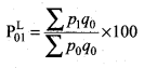
4. \(\frac{\sum p_{1} q_{1}}{\sum p_{0} q_{1}} \times 100\) is Laspeyre’s quantity index.
5. Laspeyre’s price index regards the base year quantities as fixed.

Answer:

1. True
2. True
3. False
4. False
5. True

Question 8.
Index for base period is always taken as ______
(a) 100
(b) 1
(c) 200
(d) 0
Answer:
(a) 100

Question 9.
Consumer price index indicates _______
(a) Rise
(b) Fall
(c) both (a) & (b)
(d) neither (a) & (b)
Answer:
(c) both (a) & (b)

Question 10.
The purchasing power of money can be accessed through ______
(a) simple index
(b) Fisher’s index
(c) Consumer price index (CPI)
(d) Volume index
Answer:
(c) Consumer price index (CPI)

Question 11.
For consumer price index, price quotations are collected from _______
(a) Fair price shops
(b) Government depots
(c) Retailers
(d) Whole-sale dealers
Answer:
(c) Retailers

Question 12.
The aggregative expenditure method and family budget method always give ________
(a) Different results
(b) Approximate results
(c) Same results
(d) None of these
Answer:
(c) Same results

Question 13.
The Federal Bureau of statistics prepares ________
(a) The wholesale price index
(b) CPI
(c) Sensitive price indicator
(d) All the above
Answer:
(d) All the above

Question 14.
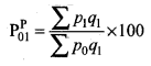
Paasche’s price index number is also called _________
(a) Base year weighted
(b) Current year weighted
(c) Simple aggregative index
(d) Consumer price index
Answer:
(b) Current year weighted

Question 15.
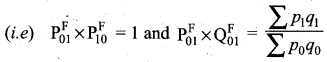
Index number calculated by Fisher’s formula is ideal because it satisfies ________
(a) Circular test
(b) Factor reversal test
(c) Time reversal test
(d) All of the above
Answer:
(d) All of the above

2 Mark Questions

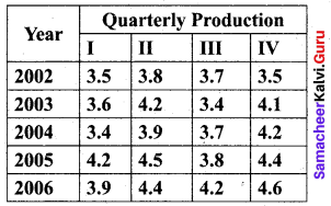
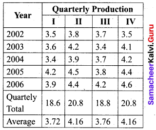
Question 1.
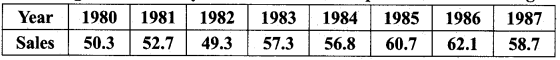
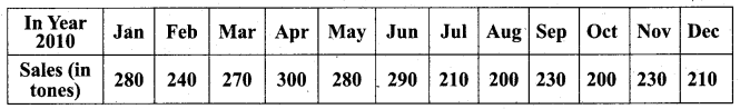
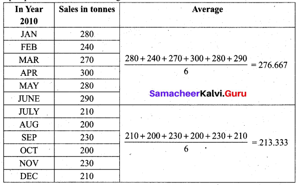
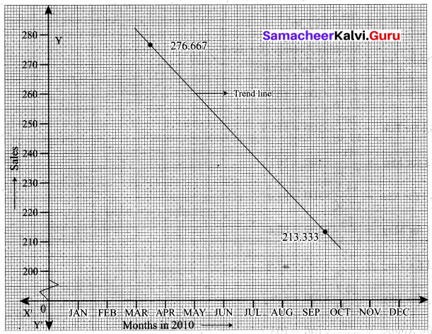
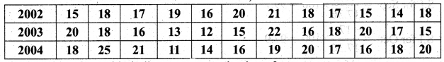
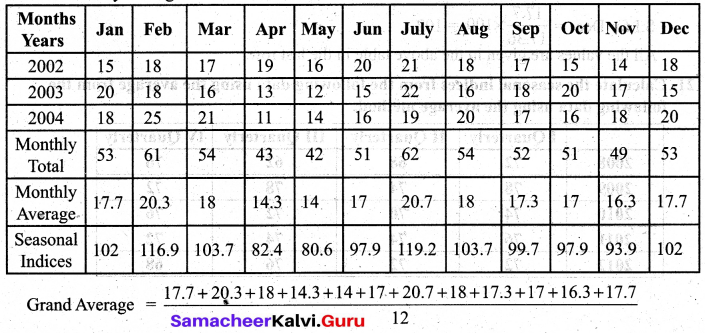
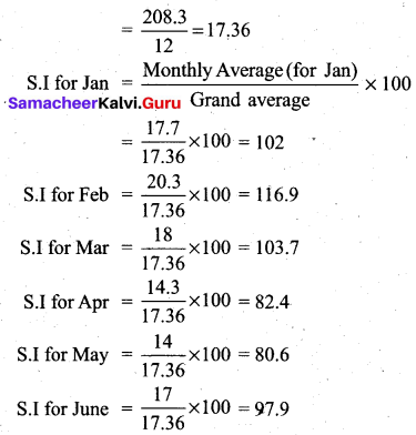
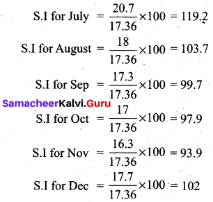
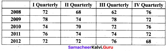
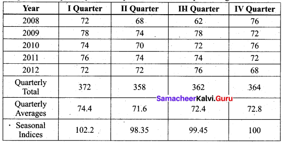
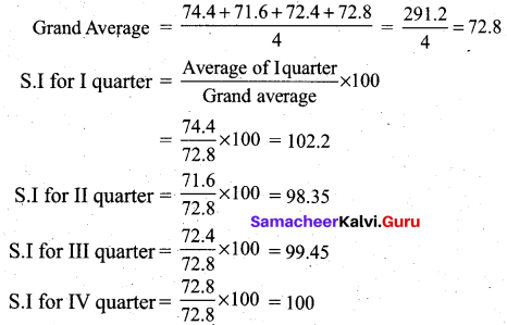
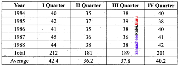
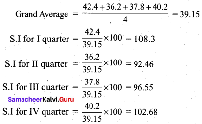
From the data given below calculate seasonal Indices:

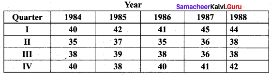
Solution:

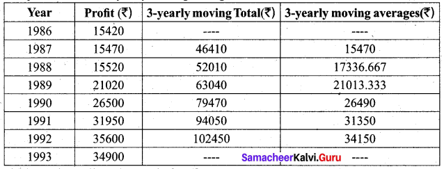
Question 2.
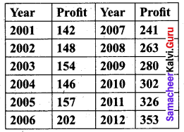
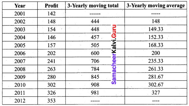
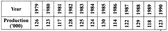
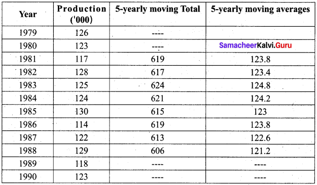
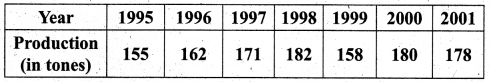
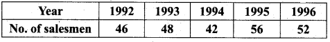
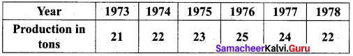
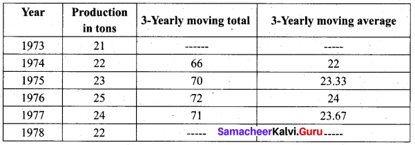
Using 3-year moving averages, determine the trend values from the following data.

Solution:

Question 3.
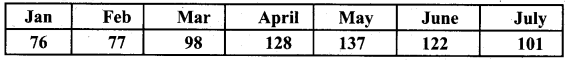
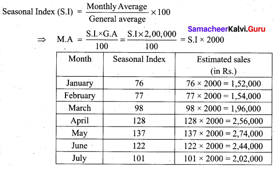
A company estimates its average monthly sales in a particular year to be Rs.2,00,000. The seasonal indices of the sales data are given below. Draw a monthly sales budget for the company.

Solution:

Question 4.
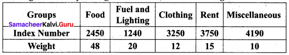
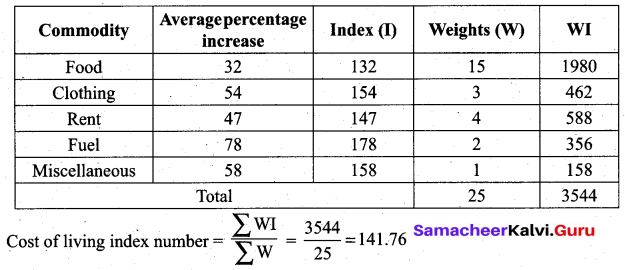
Calculate the index for the data when the average percentage increases in the prices of items and weights are given. Food 15, clothing 3, Rent 4, Fuel 2, Miscellaneous 1, the percentage increases are 32, 54, 47, 78 and 58.
Solution:

3 and 5 Marks Questions

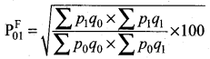
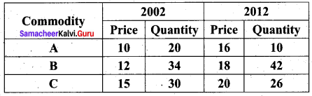
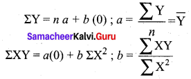
Question 1.
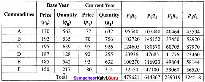
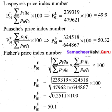
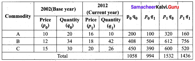
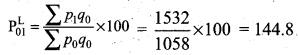
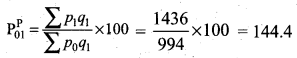
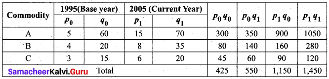
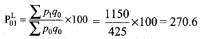
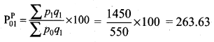
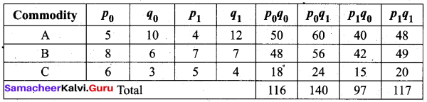
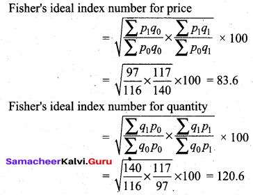
Using Fisher’s Ideal Formula, compute price and quantity index number for 1984 with 1982 as the base year, from the given information.

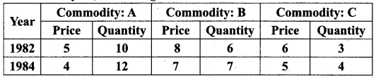
Solution:

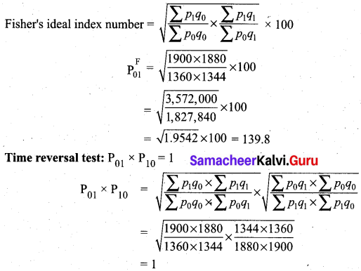
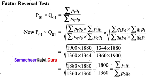
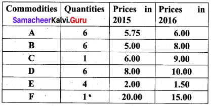
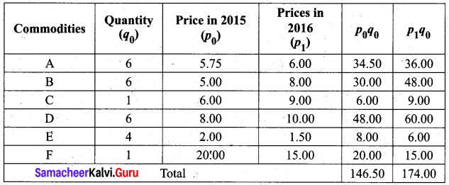
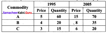
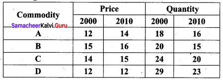
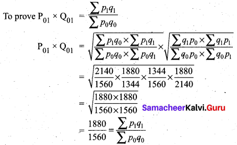
Question 2.
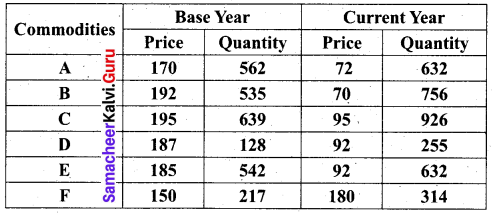
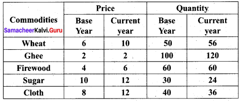
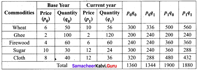
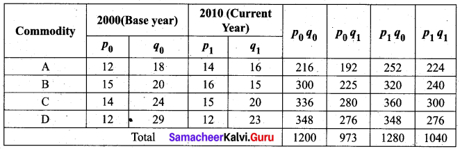
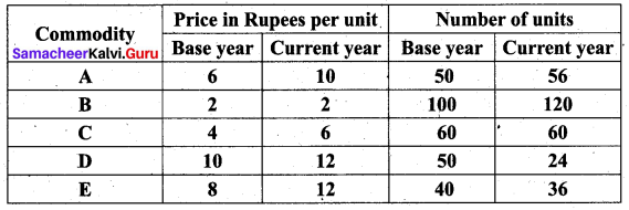
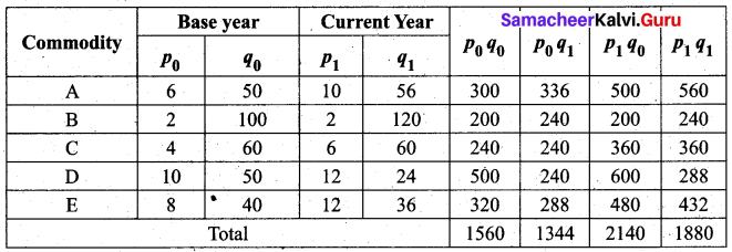
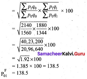
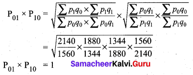
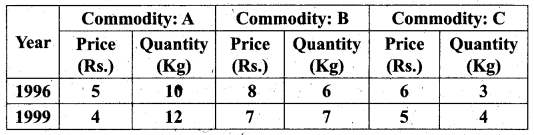
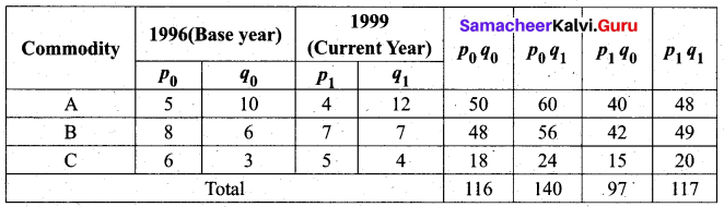
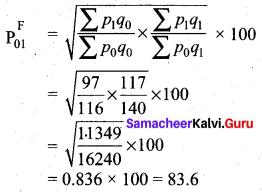
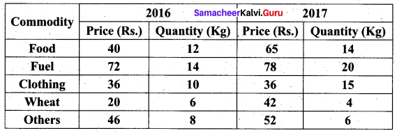
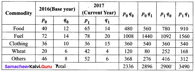
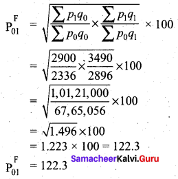
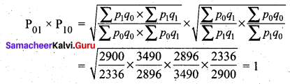
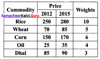
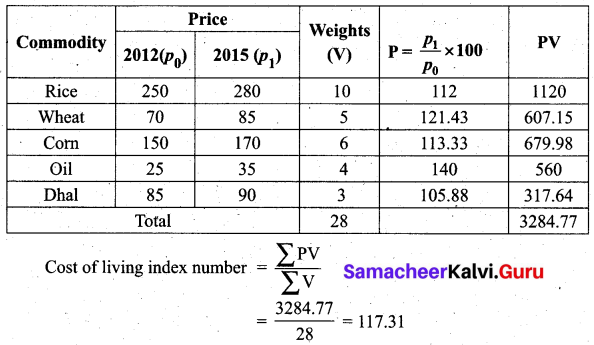
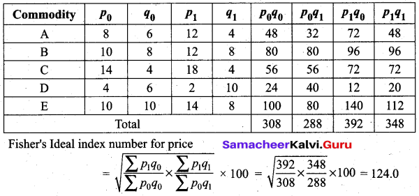
Using the following data, compute Fisher’s Ideal price index number for the current year.

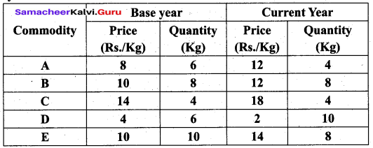
Solution:

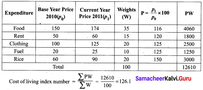
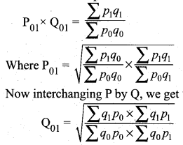
Question 3.
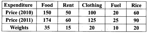
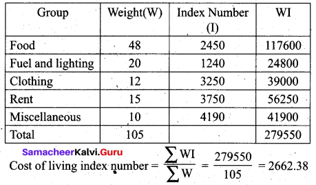
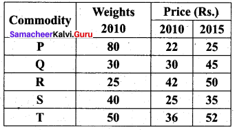
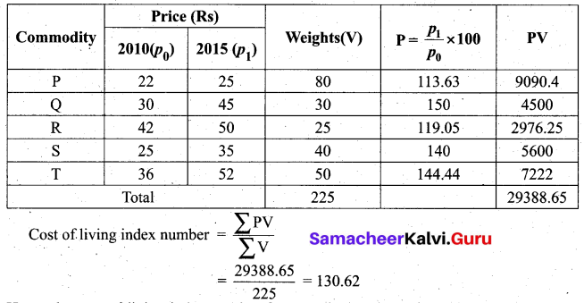
Calculate the cost of living Index number from the following data.

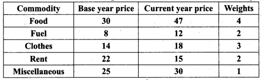
Solution:

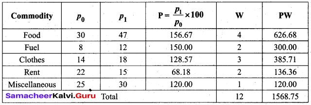
Cost of living index number = \(\frac{\sum P W}{\sum W}=\frac{1568.75}{12}\) = 130.73

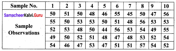
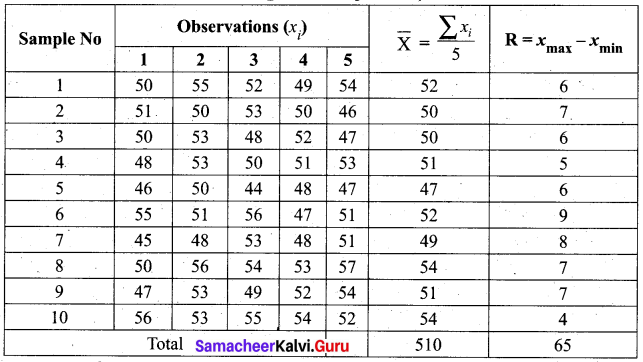
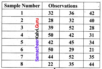
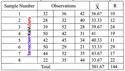
Question 4.
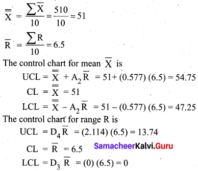
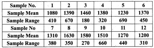
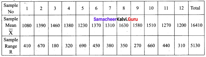
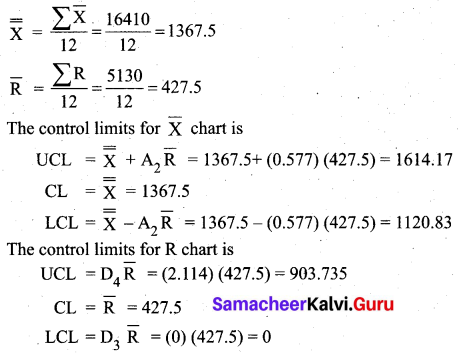
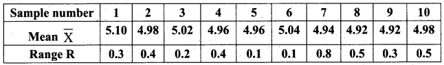
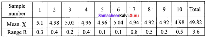
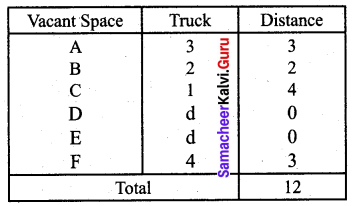
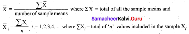
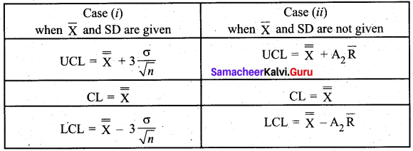
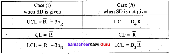
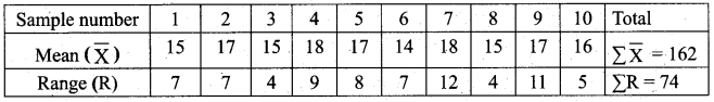
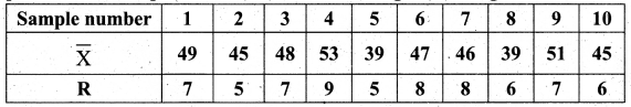
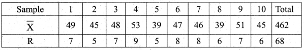
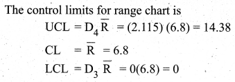
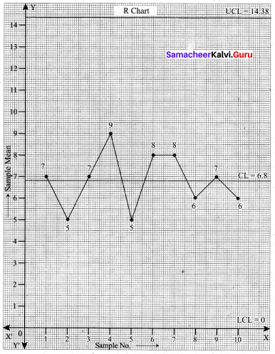
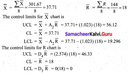
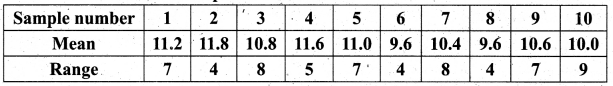
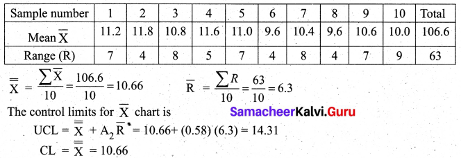
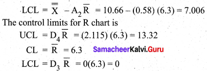
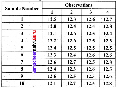
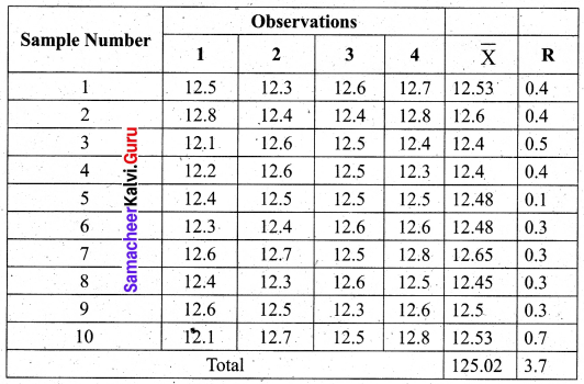
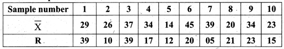
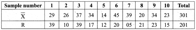
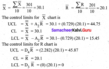
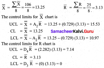
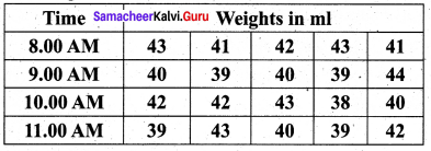
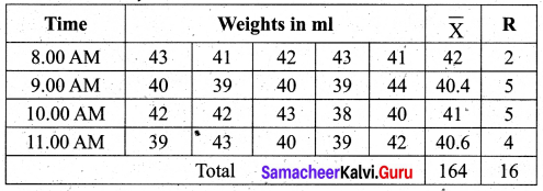
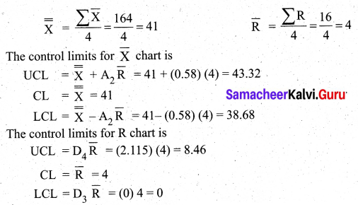
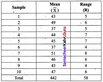
Given below are the values of the sample mean (\(\bar{X}\)) and the range (R) for ten samples of size 5 each. Find the control charts and comment on the state of the process.

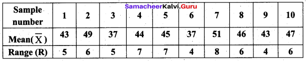
Use A₂ = 0.58, D₃ = 0, D₄ = 2.115
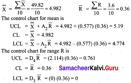
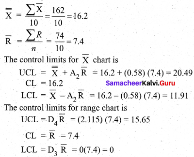
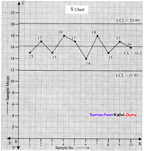
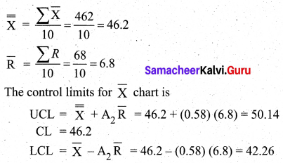
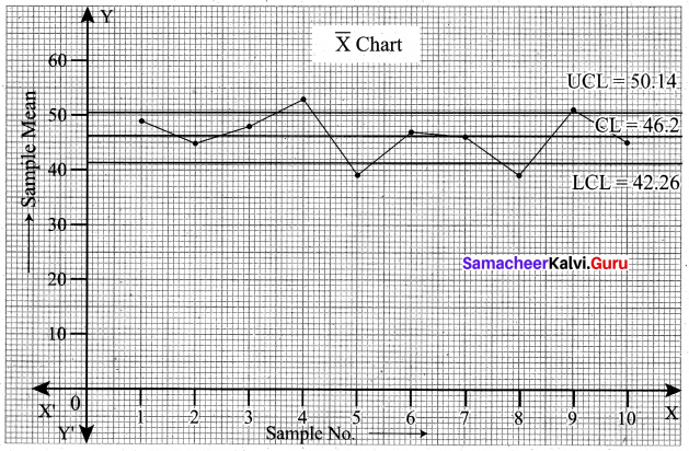
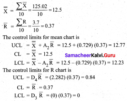
Solution:


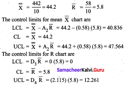
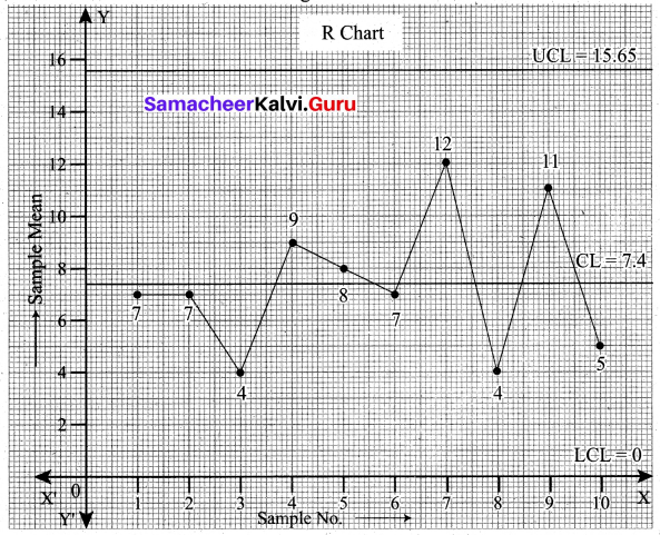
We observe that all the sample range values are within the control limits values of R chart, But two values of the sample \(\bar{X}\) (i.e) 37, 37 lies below the LCL and 49, 51 lie above the UCL. So the statistical process is out of control.

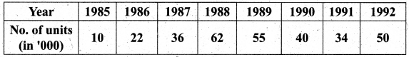
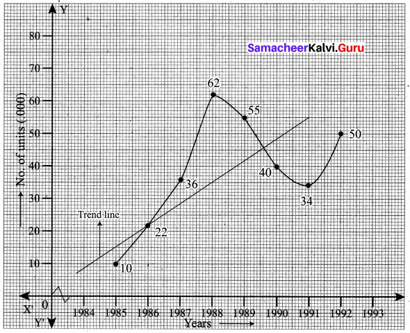
Question 5.
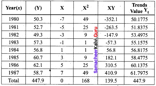
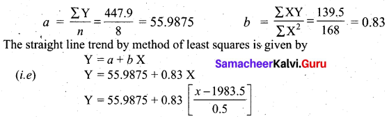
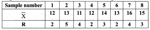
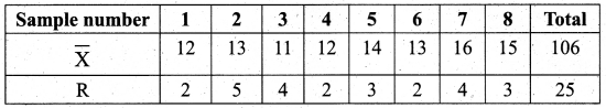
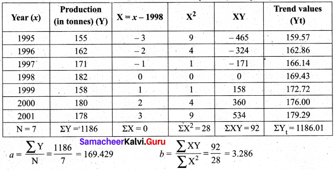
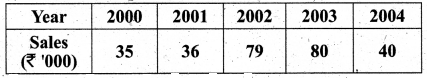
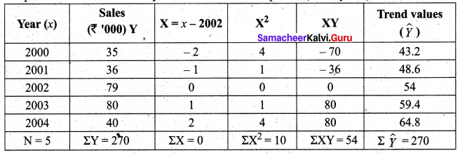
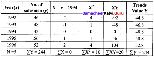
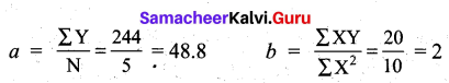
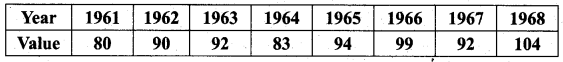
Fit a straight line trend equation by the method of least squares and estimate the trend values.

Solution:
Let Y_t = a + bx be the trend line.
Let X = \(\frac{x-1964.5}{0.5}\), x denotes year.

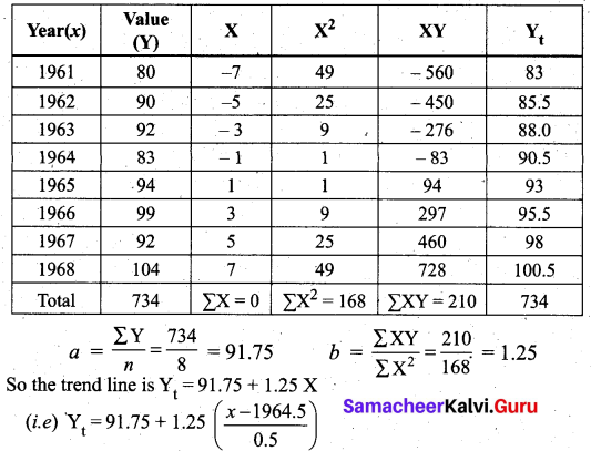
When x = 1961, Y_t = 91.75 – 7(1.25) = 83
When x = 1962, Y_t = 91.75 – 5(1.25) = 85.5
We can find other values similarly.

Students can download 12th Business Maths Chapter 9 Applied Statistics Miscellaneous Problems and Answers, Samacheer Kalvi 12th Business Maths Book Solutions Guide Pdf helps you to revise the complete Tamilnadu State Board New Syllabus and score more marks in your examinations.

Tamilnadu Samacheer Kalvi 12th Business Maths Solutions Chapter 9 Applied Statistics Miscellaneous Problems

Question 1.
Using three yearly moving averages, Determine the trend values from the following data.

Solution:

Question 2.
From the following data, calculate the trend values using fourly moving averages.

Solution:

Question 3.
Fit a straight line trend by the method of least squares to the following data.

Solution:
Let x denote the years and y denote the sales. Since number of years is even,
we take X = \(\frac{x-1983.5}{0.5}\)


The trend values are obtained by substituting the years for x, and given in the table.
When x= 1980, Y_t = 55.9875 + 0.83(-7) = 50.1775
When x = 1981, Y_t = 55.9875 – 5(0.83) = 51.8375
When x = 1982, Y_t = 55.9875 – 3(0.83) = 53.4975
When x= 1983, Y_t = 55.9875 – (0.83) = 55.1575
When x = 1984, Y_t = 55.9875 + (0.83) = 56.8175
When x = 1985, Y_t = 55.9875 + 3(0.83) = 58.4775
When x = 1986, Y_t = 55.9875 + 5(0.83) = 60.1375
When x = 1987, Y_t = 55.9875 + 7(0.83) = 61.7975
We find that ΣYt = ΣY = 447.9

Question 4.
Calculate the Laspeyre’s, Paasche’s and Fisher’s price index number for the following data. Interpret the data.

Solution:


From the index numbers, we conclude that for the same quantity, the price has reduced by 50.5% in the current year compared to the base year according to Laspeyre’s index. By the Paasche’s index number, we see that the price has reduced by 49.68% in the current year, and according to Fisher’s index number it has reduced by 49.9% in the current year.

Question 5.
Using the following data, construct Fisher’s Ideal Index Number and show that it satisfies the Factor Reversal Test and Time Reversal Test?

Solution:


This shows Fisher’s ideal index number satisfies time reversal test.

This shows Fisher’s ideal index number satisfies factor reversal test.

Question 6.
Compute the consumer price index for 2016 on the basis of 2015 from the following data.

Solution:
Consumer price index (CPI) is same as cost of living index. We use the aggregate expenditure method which gives CPI as CPI = \(\frac{\sum p_{1} q_{0}}{\sum p_{0} q_{0}} \times 100\)

Consumer price index for the year 2016 is = \(\frac{174}{146.50} \times 100\) = 118.77
On the basis of the year 2015, The cost of living has increased by 18.77%

Question 7.
An Enquiry was made into the budgets of the middle-class families in a city gave the following information.

What changes in the cost of living have taken place in the middle-class families of a city?
Solution:

For the middle-class families of the city, the cost of living has increased up to 26.1 % in 2011 as compared to 2010.

Question 8.
From the following data, calculate the control limits for the mean and range chart.

Solution:
Since the sample size is 5, we used A₂ = 0.577, D₃ = 0, D₄ = 2.114, from the table given.


We see that one sample \(\bar{X}\) value 47 is below the LCL of \(\bar{X}\). To infer that the process is not totally out of control since^the difference is less. Further investigation is recommended.

Question 9.
The following data gives the average life (in hours) and a range of 12 samples of 5 lamps each. The data are

Construct control charts for mean and range. Comment on the control limits.
Solution:
In this question the number of observations is 5 for each sample. So we use A₂ = 0.577, D₃ = 0, D₄ = 2.114 from the table of control chart constants.


We observe that the sample \(\bar{X}\) value 1080 is below the LCL. All sample range values are within the control limits for R. We say that process is out of control.

Question 10.
The following are the sample means and ranges for 10 samples, each of size 5. Calculate the control limits for the mean chart and range chart and state whether the process is in control or not.

Solution:


We observe that all sample \(\bar{X}\) values are within the control limits value of \(\bar{X}\) chart. But the sample range value 0.8 is above the UCL of the R chart. So we conclude that the process is out of control.

Students can download 12th Business Maths Chapter 10 Operations Research Ex 10.3 Questions and Answers, Samacheer Kalvi 12th Business Maths Book Solutions Guide Pdf helps you to revise the complete Tamilnadu State Board New Syllabus and score more marks in your examinations.

Tamilnadu Samacheer Kalvi 12th Business Maths Solutions Chapter 10 Operations Research Ex 10.3

Question 1.
Given the following pay-off matrix (in rupees) for three strategies and two states of nature.

Select a strategy using each of the following rule (i) Maximin (ii) Minimax
Solution:
(i) Maximin principle

Max (40, -20, -40) = 40. Since the maximum pay-off is Rs.40, the best strategy is S₁ according to maximin rule.
(ii) Minimax principle

Min (60, 10, 150) = 10. Since the minimum pay- off is Rs. 10, the best strategy is S₂ according to minimax rule.

Question 2.
A farmer wants to decide which of the three crops he should plant on his 100-acre farm. The profit from each is dependent on the rainfall during the growing season. The farmer has categorized the amount of rainfall as high, medium and low. His estimated profit for each is shown in the table.

If the farmer wishes to plant the only crop, decide which should be his best crop using (i) Maximin (ii) Minimax
Solution:
(i) Maximin principle

Max (2000, 3500, 4000) = 4000. Since the maximum profit is Rs. 4000, he must choose crop C as the best crop.
(ii) Minimax principle

Min (8000, 5000, 5000) = 5000. Since the minimum cost is Rs.5000, he can choose crop B and crop C as the best crop.

Question 3.
The research department of Hindustan Ltd. has recommended paying the marketing department to launch a shampoo of three different types. The marketing types of shampoo to be launched under the following estimated pay-offs for various level of sales.

What will be the marketing manager’s decision if (i) Maximin and (ii) Minimax principle applied?
Solution:
(i) Maximin principle

Max (10, 5, 3) = 10. Since the maximum pay-off is 10 units, the marketing manager has to choose Egg shampoo by Maximin rule.
(ii) Minimax principle

Min (30, 40, 55) = 30. Since the minimum pay-off is 30 units, the marketing manager has to choose Egg shampoo by minimax rule.

Question 4.
Following pay-off matrix, which is the optimal decision under each of the following rule (i) Maximin (ii) Minimax

Solution:
(i) Maximin principle

Max (5, 7, 9, 8) = 9. Since the maximum pay-off is 9, the optimal decision is A₃ according to maximin rule.
(ii) Minimax principle

Min (14, 11, 11, 13) = 11. Since the minimum pay-off is 11, the optimal decision A₂ and A₃ according to minimax rule.

Students can download 12th Business Maths Chapter 9 Applied Statistics Ex 9.4 Questions and Answers, Samacheer Kalvi 12th Business Maths Book Solutions Guide Pdf helps you to revise the complete Tamilnadu State Board New Syllabus and score more marks in your examinations.

Tamilnadu Samacheer Kalvi 12th Business Maths Solutions Chapter 9 Applied Statistics Ex 9.4

Choose the correct answer.

Question 1.
A time series is a set of data recorded _______
(a) Periodically
(b) Weekly
(c) Successive points of time
(d) all the above
Answer:
(d) all the above

Question 2.
A time series consists of ________
(a) Five components
(b) Four components
(c) Three components
(d) Two components
Answer:
(b) Four components

Question 3.
The components of a time series which is attached to short term fluctuation are _______
(a) Secular trend
(b) Seasonal variations
(c) Cyclic variation
(d) Irregular variation
Answer:
(d) Irregular variation

Question 4.
Factors responsible for seasonal variations are ______
(a) Weather
(b) Festivals
(c) Social customs
(d) All the above
Answer:
(d) All the above

Question 5.
The additive model of the time series with the components T, S, C and I is _______
(a) y = T + S + C × I
(b) y = T + S × C × I
(c) y = T + S + C + I
(d) y = T + S × C + I
Answer:
(c) y = T + S + C + I

Question 6.
Least square method of fitting a trend is _______
(a) Most exact
(b) Least exact
(c) Full of subjectivity
(d) Mathematically unsolved
Answer:
(a) Most exact

Question 7.
The value of ‘b’ in the trend line y = a + bx is _________
(a) Always positive
(b) Always negative
(c) Either positive or negative
(d) Zero
Answer:
(c) Either positive or negative

Question 8.
The component of a time series attached to long term variation is trended as _______
(a) Cyclic variation
(b) Secular variations
(c) Irregular variation
(d) Seasonal variations
Answer:
(b) Secular variations

Question 9.
The seasonal variation means the variations occurring within ________
(a) A number of years
(b) within a year
(c) within a month
(d) within a week
Answer:
(b) within a year

Question 10.
Another name of the consumer’s price index number is _______
(a) Whole-sale price index number
(b) Cost of living index
(c) Sensitive
(d) Composite
Answer:
(b) Cost of living index

Question 11.
Cost of living at two different cities can be compared with the help of _______
(a) Consumer price index
(b) Value index
(c) Volume index
(d) Un-weighted index
Answer:
(a) Consumer price index

Question 12.
Laspeyre’s index = 110, Paasche’s index = 108, then Fisher’s Ideal index is equal to _______
(a) 110
(b) 108
(c) 100
(d) 109
Answer:
(d) 109
Hint:
Fisher’s Index = \(\sqrt{110 \times 108}\) = 109

Question 13.
Most commonly used index number is _________
(a) Volume index number
(b) Value index number
(c) Price index number
(d) Simple index number
Answer:
(c) Price index number

Question 14.
Consumer price index are obtained by ________
(a) Paasche’s formula
(b) Fisher’s ideal formula
(c) Marshall Edgeworth formula
(d) Family budget method formula
Answer:
(d) Family budget method formula

Question 15.
Which of the following Index number satisfy the time-reversal test?
(a) Laspeyre’s Index number
(b) Paasche’s Index number
(c) Fisher’s Index number
(d) All of them
Answer:
(c) Fisher’s Index number

Question 16.
While computing a weighted index, the current period quantities are used in the _______
(a) Laspeyre’s method
(b) Paasche’s method
(c) Marshall Edgeworth method
(d) Fisher’s ideal method
Answer:
(b) Paasche’s method

Question 17.
The quantities that can be numerically measured can be plotted on a ________
(a) p – chart
(b) c – chart
(c) x bar chart
(d) np – chart
Answer:
(c) x bar chart

Question 18.
How many causes of variation will affect the quality of a product?
(a) 4
(b) 3
(c) 2
(d) 1
Answer:
(c) 2

Question 19.
Variations due to natural disorder is known as _______
(a) random cause
(b) non-random cause
(c) human cause
(d) all of them
Answer:
(a) random cause

Question 20.
The assignable causes can occur due to _______
(a) poor raw materials
(b) unskilled labour
(c) faulty machines
(d) all of them
Answer:
(d) all of them

Question 21.
A typical control charts consists of ________
(a) CL, UCL
(b) CL, LCL
(c) CL, LCL, UCL
(d) UCL, LCL
Answer:
(c) CL, LCL, UCL

Question 22.
\(\bar{X}\) chart is a ______
(a) attribute control chart
(b) variable control chart
(c) neither Attribute nor variable control chart
(d) both Attribute and variable control chart
Answer:
(b) variable control chart

Question 23.
R is calculated using ______
(a) \(x_{\max }-x_{\min }\)
(b) \(x_{\min }-x_{\max }\)
(c) \(\bar{x}_{\max }-\bar{x}_{\min }\)
(d)
Answer:
(a) \(x_{\max }-x_{\min }\)

Question 24.
The upper control limit for \(\bar{X}\) chart is given by _______
(a) \(\overline{\mathrm{X}}+\mathrm{A}_{2} \overline{\mathrm{R}}\)
(b)
(c)
(d)
Answer:
(c)

Question 25.
The LCL for R chart is given by ________
(a) \(\mathrm{D}_{2} \overline{\mathrm{R}}\)
(b)
(c)
(d) \(\mathbf{D}_{3} \overline{\mathbf{R}}\)
Answer:
(d) \(\mathbf{D}_{3} \overline{\mathbf{R}}\)

Students can download 12th Business Maths Chapter 10 Operations Research Ex 10.2 Questions and Answers, Samacheer Kalvi 12th Business Maths Book Solutions Guide Pdf helps you to revise the complete Tamilnadu State Board New Syllabus and score more marks in your examinations.

Tamilnadu Samacheer Kalvi 12th Business Maths Solutions Chapter 10 Operations Research Ex 10.2

Question 1.
What is the Assignment problem?
Solution:
Suppose that we have ‘m’ jobs to be performed on ‘n’ machines. The cost of assigning each job to each machine is C_ij. (i = 1, 2,…, n and j = 1, 2,…. n).Our objective is to assign different jobs to different machines (one job per machine) to minimize the overall cost. This is known as the assignment problem.

Question 2.
Give the mathematical form of the assignment problem.
Solution:
The mathematical form of assignment problem is Minimize \(\mathrm{Z}=\sum_{i=1}^{n} \sum_{j=1}^{n} \mathrm{C}_{i j} x_{i j}\)
Subject to the constraints

(or) 1 for all i = 1, 2, …….. n and j = 1, 2, …….. n
where C_ij is the cost of assigning ith job to jth machine and x_ij represents the assignment of ith job to jth machine.

Question 3.
What is the difference between Assignment Problem and Transportation Problem?
Solution:
The assignment problem is a special case of the transportation problem. The differences are given below.

Transportation Problem	Assignment Problem
1. This is about reducing cost of transportation merchandise	1. This is about assigning finite sources to finite destinations where only one destination is allotted for one source with minimum cost
2. Number of sources and number of demand need not be equal	2. Number of sources and the number of destinations must be equal
3. If total demand and total supply are not equal then the problem is said to be unbalanced.	3. If the number of rows are not equal to the number of columns then problems are unbalanced.
4. It requires 2 stages to solve: Getting initial basic feasible solution, by NWC, LCM, VAM and optimal solution by MODI method	4. It has only one stage. Hungarian method is sufficient for obtaining an optimal solution

Question 4.
Three jobs A, B and C one to be assigned to three machines U, V and W. The processing cost for each job machine combination is shown in the matrix given below. Determine the allocation that minimizes the overall processing cost. (cost is in ₹ per unit)

Solution:
Here the number of rows and columns are equal.
the given assignment problem is balance.
Step 1: We select the smallest element from each row and subtract from other elements in its row.

Column V has no zero. Go to step 2.
Step 2: Select the smallest element from each column and subtract from other elements in its column.

Since each row and column contains at least one zero, assignments can be made.
Step 3: (Assignment)
Row A contains exactly one zero. We mark it by □ and other zeros in its column by x.

Now proceed column wise. Column V has exactly one zero. Mark by □ and other zeros in its row by X.

Now there is no zero in row B to assign the job. So proceed as follows. Draw a minimum number of lines to cover all the zeros in the reduced matrix. Subtract 5 from all the uncovered elements and add to the element at the intersection of 2 lines as shown below.

Now start the whole procedure once again for assignment to get the following matrix.

Thus all the 3 assignments have been made. The optimal assignment schedule and the total cost is
Job Machine Cost

Question 5.
A computer centre has got three expert programmers. The centre needs three application programmes to be developed. The head of the computer centre, after studying carefully the programmes to be developed, estimates the computer time in minutes required by the experts to the application programme as follows.

Assign the programmers to the programme in such a way that the total computer time is least.
Solution:
Here the number of rows equals the number of columns. So the given problem is balanced and we can find a solution.
Step 1:

Step 2:

Step 3: (Assignment)

Now all the 3 programmes have been assigned to the programmers. The optimal assignment schedule and the total cost is

The optimal assignment (minimum) cost is ₹ 280.

Question 6.
A departmental head has four subordinates and four tasks to be performed. The subordinates differ inefficiency and the tasks differ in their intrinsic difficulty. His estimates of the time each man would take to perform each task is given below

How should the tasks be allocated to subordinates so as to minimize the total man-hours?
Solution:
A number of tasks equal the number of subordinates. So the given problem is balanced and we can get an optimal solution.
Step 1: Subtract minimum hours of each row from other elements of that row.

Since column 2 has no zero, proceed further.
Step 2:

We can proceed with the assignment since all the rows and columns have zeros.
Step 3: (Assignment)

Now there is no zero in row S. So we proceed as below.

We have drawn the minimum number of lines to cover all the zeros in the reduced matrix obtained. The smallest element from all the uncovered elements is 1. We subtract this from all the uncovered elements and add them to the elements which lie at the intersection of two lines. Thus we obtain another reduced problem for fresh assignment.

Now all the subordinates have been assigned tasks. The optimal assignment schedule and the total cost is

The optimal assignment (minimum) hours = 41

Question 7.
Find the optimal solution for the assignment problem with the following cost matrix.

Solution:
Number of Areas = Number of salesmen.
So the given problem is balanced and we can find an optimal solution.
Step 1:

Step 2:

Step 3: (Assignment)

Now all the salesmen have been assigned areas.
The optimal assignment schedule and the total cost is

Thus the optimal cost is Rs. 37.

Question 8.
Assign four trucks 1, 2, 3 and 4 to vacant spaces A, B, C, D, E and F so that distance travelled is minimized. The matrix below shows the distance.

Solution:
Here the number of trucks is 4 and vacant spaces are 6. So the given assignment problem is the unbalanced problem. So we introduce two dummy columns with all the entries zero to make is balanced. So the problem is

Here only 4 vacant spaces can be assigned to four trucks
Step 1: Not necessary since all rows have zeros.
Step 2:

Step 3: (Assignment)

The optimal assignment schedule and total distance travelled is

Thus the minimum distance travelled is 12 km.

Students can download 12th Business Maths Chapter 9 Applied Statistics Ex 9.3 Questions and Answers, Samacheer Kalvi 12th Business Maths Book Solutions Guide Pdf helps you to revise the complete Tamilnadu State Board New Syllabus and score more marks in your examinations.

Tamilnadu Samacheer Kalvi 12th Business Maths Solutions Chapter 9 Applied Statistics Ex 9.3

Question 1.
Define Statistical Quality Control.
Solution:
Statistical quality control (SQC) refers to the use of statistical methods in the monitoring and maintaining of the quality of products and services. This method is used to determine the tolerance limits for accepting a production process.

Question 2.
Mention the types of causes for variation in a production process.
Solution:
There are two causes of variations between items produced under identical conditions in large production process. They are called assignable causes and non-assignable causes (chance causes).

Question 3.
Define Chance Cause.
Solution:
The minor causes which do not affect the quality of the products to an extent are called as chance causes or Random causes. For example rain, floods, power cuts, etc.

Question 4.
Define Assignable Cause.
Solution:
The variations in input factors which are the causes for the variations in the output produc¬tions are called assignable causes. For example defective raw materials, fault in instruments used, fatigue of workers employed, unskilled technicians, worn out tools etc.

Question 5.
What do you mean by product control?
Solution:
Product control means controlling the quality of the product by a sampling technique called acceptance sampling. It aims at a certain quality level to he guaranteed to the customers. It is concerned with classification of raw materials, semi-finished goods or finished goods into acceptable or rejectable products.

Question 6.
What do you mean by process control?
Solution:
A production process is said to be under control if the products produced are according to the specifications; that is the characteristics are within the tolerance limits. This is tested through the control charts.

Question 7.
Define a control chart.
Solution:
Control charts are statistical tools to test whether a production process is under control. It was introduced by Watter.A.Shewhart. It is a simple technique used for detecting patterns of variations in the data. It consists of three lines namely, centre line (CL), Upper control limit (UCL) and Lower control limit (LCL)

Question 8.
Name the control charts for variables.
Solution:
A quality characteristic which can be expressed in terms of a numerical value in the production process is called as a variable. There are two types of control charts for variables.

1. Mean chart (\(\bar{X}\) chart)
2. Range chart (R chart).

Question 9.
Define the mean chart.
Solution:
The mean chart (\(\bar{X}\) chart) is used to show the quality averages of the samples taken from the given process. The mean of the samples is first calculated. Then the mean of the sample means is found to get the control limits.

Question 10.
Define R Chart.
Solution:
The R chart is used to show the variability or dispersion of the samples taken from the given process. The average range is given by \(\overline{\mathrm{R}}=\frac{\sum R}{n}\), where R = x_max – x_min for each ‘n’ samples. For samples of size less than 20, the range provides a good estimate of σ. Hence to measure the variance in the variable, range chart is used.

Question 11.
What are the uses of statistical quality control?
Solution:
The term Quality means a level or standard of a product which depends on Material, Manpower, Machines, and Management (4M’s). Quality Control ensures the quality specifications all along with them from the arrival of raw materials through each of their processing to the final delivery of goods. This technique is used in almost all’ production industries such as automobile, textile, electrical equipment, biscuits, bath soaps, chemicals, petroleum products etc.

Question 12.
Write the control limits for the mean chart.
Solution:
The calculation of control limits for \(\bar{X}\) chart in two different cases are

Question 13.
Write the control limits for the R chart.
Solution:
The calculation of control limits for R chart in two different cases are

Question 14.
A machine is set to deliver packets of a given weight. Ten samples of size five each were recorded. Below are given relevant data:

Calculate the control limits for the mean chart and the range chart and then comment on the state of control.
(conversion factors for n = 5, A₂ = 0.58, D₃ = 0 and D₄ = 2.115)
Solution:



The above diagram shows all the three control lines with the data points plotted. We see that all the points of the sample mean are within the control limits.
We now draw the R chart for the given data.

The above diagram shows all the three control lines with the sample range points plotted. We observe that all the points are within the control limits.
Conclusion: From the above two plots of the sample mean \(\bar{X}\) and sample range R, we conclude that the process is in control.

Question 15.
Ten samples each of size five are drawn at regular intervals from a manufacturing process. The sample means (\(\bar{X}\)) and their ranges (R) are given below:

Calculate the control limits in respect of \(\bar{X}\) chart.
(Given A₂ = 0.58, D₃ = 0 and D₄ = 2.115) Comment on the state of control
Solution:





From the \(\bar{X}\) chart, we see that 4 points are outside the control limit lines. So we say that the process is out of control.

Question 16.
Construct \(\bar{X}\) and R charts for the following data:

(Given for n = 3, A₂ = 1.023, D₃ = 0 and D₄ = 2.574)
Solution:
We first find the sample mean and range for each of the 8 given samples.

Question 17.
The following data show the values of the sample mean (\(\bar{X}\)) and its range (R) for the samples of Size five each. Calculate the values for control limits for mean, range chart and determine whether the process is in control.

(conversion factors for n = 5, A₂ = 0.58, D₃ = 0 and D₄ = 2.115)
Solution:


From the above control limits values we observe that all the sample means lie between the UCL and LCL (i.e.) 7.006 < \(\overline{\mathrm{x}}_{i}\) < 14.31 for i = 1, 2, 3,…….. 10. Also all the sample range value lie between the control limits for R (i.e) 0 < R_i < 13.32, i = 1, 2, 3,…., 10. Hence we conclude that the process is in control.

Question 18.
A quality control inspector has taken ten samples of size four packets each from a potato chips company. The contents of the sample are given below, Calculate the control limits for the mean and range chart.

(Given for n = 4, A₂ = 0.729, D₃ = 0 and D₄ = 2.282)
Solution:

Question 19.
The following data show the values of sample means and the ranges for ten samples of size 4 each. Construct the control chart for mean and range chart and determine whether the process is in control

Solution:


From the values of the control limits for \(\bar{X}\), we observe that one sample \(\bar{X}\) value (45) is above the UCL and one sample \(\bar{X}\) value (14) is below the LCL. Hence we conclude that the process is out of control.

Question 20.
In a production process, eight samples of size 4 are collected and their means and ranges are given below. Construct a mean chart and range chart with control limits.

Solution:


From the values of the control limits for \(\bar{X}\), we observe that sample \(\bar{X}\) value 16 is above the UCL. Hence we conclude that the process is out of control.

Question 21.
In a certain bottling industry, the quality control inspector recorded the weight of each of the 5 bottles selected at random during each hour of four hours in the morning.

Solution:


From the above control limit values. We observe that all the sample \(\bar{X}\) values are within UCL and LCL values. Also, all the R values are also within UCL and LCL of R chart. Hence we conclude that the process is within Control.

Students can download 12th Business Maths Chapter 9 Applied Statistics Ex 9.2 Questions and Answers, Samacheer Kalvi 12th Business Maths Book Solutions Guide Pdf helps you to revise the complete Tamilnadu State Board New Syllabus and score more marks in your examinations.

Tamilnadu Samacheer Kalvi 12th Business Maths Solutions Chapter 9 Applied Statistics Ex 9.2

Question 1.
Define Index Number.
Solution:
“An Index Number is a device which shows by its variations the Changes in a magnitude which is not capable of accurate measurements in itself or of direct valuation in practice”. – Wheldon

“An Index number is a statistical measure of fluctuations in a variable arranged in the form of a series and using a base period for making comparisons” – Lawrence J Kalpan

Question 2.
State the uses of Index Number.
Solution:
The uses of Index number are as given below:

• It is an important tool for formulating decision and management policies.
• It helps in studying the trends and tendencies.
• It determines the inflation and deflation in an economy

Question 3.
Mention the classification of Index Number.
Solution:
Classification of Index Numbers:
Index number can be classified as follows

1. Price Index Number: It measures the general changes in the retail or wholesale price level of a particular or group of commodities.
2. Quantity Index Number: These are indices to measure the changes in the number of goods manufactured in a factory.
3. Cost of living Index Number: These are intended to study the effect of change in the price level on the cost of living of different classes of people.

Question 4.
Define Laspeyre’s price index number
Solution:
The weighted aggregate index number using base period weights is called Laspeyre’s price index number.

Where p₁ is current year price
p₀ is base year price
q₀ is base year quantity

Question 5.
Explain Paasche’s price index number.
Solution:
If both prices and quantities were permitted to change, then it is impossible to isolate the part of movement due to price changes alone. In this case, the current year quantities appear more realistic weights than the base year quantities. The index number based on current year quantities is called Paasche’s price index number.

Where p₁ is the current year price
q₁ is the current year quantity
p₀ is the base year price

Question 6.
Write a note on Fisher’s price index number.
Solution:
Fisher defined a weighted index number as the geometric mean of Laspeyre’s index number and Paasche’s Index number

The Fisher-price index number is also known as the “ideal” price index number. This requires more data than the other two index numbers and as a result, may often be impracticable. But this is a good index number because it satisfies both the time-reversal test and factor reversal test.

Question 7.
State the test of the adequacy of the index number.
Solution:
Index numbers are studied to know the- relative changes in price and quantity for any two years compared. There are two tests which are used to test the adequacy for an index number. The two tests are as follows

• Time Reversal Test
• Factor Reversal Test

The criterion for a good index number is to satisfy the above two tests.

Question 8.
Define Time Reversal Test.
Solution:
It is an important test for testing the consistency of a good index number. This test maintains time consistency by working both forward and backward with respect to time (here time refers to the base year and current year). Symbolically the following relationship should be satisfied, P₀₁ × P₁₀ = 1
Fisher’s index number formula satisfies the above relationship

when the base year and current year are interchanged, we get,

Question 9.
Explain Factor Reversal Test.
Solution:
Factor Reversal Test:
This is another test for testing the consistency of a good index number. The product of price index number and quantity index number from the base year to the current year should be equal to the true value ratio. That is the ratio between the total value of the current period and total value pf the base period is known as the true value ratio. Factor Reversal Test is given by,

where P₀₁ is the relative change in price.
Q₀₁ is the relative change in quantity.

Question 10.
Define true value ratio.
Solution:
The ratio between the total value of the current period and the total value of the base period is known as the true value ratio.
(i.e) true value ratio = \(\frac{\sum p_{1} q_{1}}{\sum p_{0} q_{0}}\)

Question 11.
Discuss Cost of Living Index Number.
Solution:
Cost of Living Index Number is constructed to study the effect of changes in the price of goods and services of consumers for a current period as compared with the base period. The change in the cost of living index number between any two periods means the change in income which will be necessary to maintain the same standard of living in both the periods. Therefore the cost of living index number measures the average increase in the cost to maintain the same standard of life.

Further, the consumption habits of people differ widely from class to class (rich, poor, middle class) and even with the region. The changes in the price level affect the different classes of people, consequently, the general price index numbers fail to reflect the effect of changes in their cost of living in different classes of people. Therefore, the cost of living index number measures the general price movement of the commodities consumed by different classes of people.

Question 12.
Define Family Budget Method.
Solution:
Family Budget Method:
In this method, the weights are calculated by multiplying prices and quantity of the base year.
(i.e.) V = Σp₀q₀. The formula is given by,
Cost of Living Index Number = \(\frac{\sum \mathrm{PV}}{\sum \mathrm{V}}\)
where P = \(\frac{p_{1}}{p_{0}} \times 100\) is the price relative
V = Σp₀q₀ is the value relative

Question 13.
State the uses of the Cost of Living Index Number.
Solution:
Uses of Cost of Living Index Number

• It indicates whether the real wages of workers are rising or falling for a given time.
• It is used by the administrators for regulating dearness allowance or grant of bonus to the workers.

Question 14.
Calculate by a suitable method, the index number of price from the following data:

Solution:

The Laspeyres price index number

Paasche’s price index number

On an average, there is an increase of 44.8% and 44.4% in the price of the commodities by Laspeyres and Paasche’s price index number respectively for the current year 2012 as compared with the base year 2002.

Question 15.
Calculate price index number for 2005 by (a) Laspeyre’s (b) Paasche’s method.

Solution:

Laspeyre’s price index number

Paasche’s price index number

On an average, there is an increase of 170.6% and 163.63% in the price of the commodities by Laspeyre’s and Paasche’s price index number respectively for the current year 2005 as compared with the base year 1995.

Question 16.
Compute (i) Laspeyre’s (ii) Paasche’s (iii) Fisher’s Index numbers for 2010 from the following data.

Solution:

Laspeyre’s price index number

Paasche’s price index number

Fisher’s price index number

On an average, there is an increase of 6.6%, 6.8% and 6.7% in the price of the commodities by Laspeyre’s, Paasche’s and Fisher’s index number respectively for the current year 2010 as compared to the base year 2000.

Question 17.
Using the following data, construct Fisher’s Ideal index and show how it satisfies Factor Reversal Test and Time Reversal Test?

Solution:

Fisher’s ideal index

Time reversal test:
To prove P₀₁ × P₁₀ = 1

Time reversal test is satisfied.

Factor Reversal Test:

Factor Reversal Test is satisfied.

Question 18.
Using Fisher’s Ideal Formula; compute price index number for 1999 with 1996 as the base year, given the following.

Solution:

Fisher’s index number

Thus we interpret that on an average, there is a decrease of 16.41 % in the price of commodities by Fisher’s Index number for the current year 1999 as compared to the base year 1996.

Question 19.
Calculate Fisher’s index number to the following data. Also, show that satisfies Time Reversal Test.

Solution:

Fisher’s price index number

On average, there is an increase of 22.3% in the price of commodities by Fisher’s Index number for the current year 2017 as compared to the base year 2016
Time reversal test:
To prove P₀₁ × P₁₀ = 1

Time reversal test is satisfied.

Question 20.
The following are the group index numbers and the group weights of an average working-class family’s budget. Construct the cost of living index number:

Solution:

Question 21.
Construct the cost of living Index number for 2015 on the basis of 2012 from the following data using the family budget method.

Solution:

Hence, the cost of living index number for a particular class of people for the year 2015 is increased by 17.31% as compared to the year 2012.

Question 22.
Calculate the cost of living index by aggregate expenditure method:

Solution:

Hence, the cost of living index number for a particular class of people for the year 2015 is increased by 30.62% as compared to the year 2010.

Students can download 12th Business Maths Chapter 10 Operations Research Ex 10.1 Questions and Answers, Samacheer Kalvi 12th Business Maths Book Solutions Guide Pdf helps you to revise the complete Tamilnadu State Board New Syllabus and score more marks in your examinations.

Tamilnadu Samacheer Kalvi 12th Business Maths Solutions Chapter 10 Operations Research Ex 10.1

Question 1.
What is the transportation problem?
Solution:
The transportation problem deals with transporting goods from a source to a destination by minimum cost.
Description: A Manufacturer has a number of factories which produces goods at a fixed rate. He also has a number of warehouses, each of which has a fixed storage capacity. There is a cost to transport goods from a factory to a warehouse. Find the transportation of goods from factory to the warehouse that has the lowest possible cost.
Example:
Factories:
A₁ makes 5 units
A₂ makes 4 units
A₃ makes 6 units
Warehouses:
b₁ can store 5 units
b₂ can store 3 units
b₃ can store 5 units
b₄ can store 2 units
Transportation costs:

Question 2.
Write the mathematical form of transportation problem.
Solution:
Mathematically a transportation problem is nothing but a special linear programming problem in which the objective function is to minimize the cost of transportation subjected to the demand and supply constraints.
Let there be ‘m’ sources of supply having ‘a_i‘ units of supplies respectively to be transported among ‘n’ destinations with ‘b_j‘ units of requirements respectively. Let C_ij be the cost of shipping one unit of the commodity from source i to destination j for each route. Let x_ij be the units shipped per route.
Then the LPP is stated below.

Question 3.
What are a feasible solution and non-degenerate solution in the transportation problem?
Solution:
Feasible Solution: A feasible solution to a transportation problem is a set of non-negative values x_ij (i = 1, 2,.., m, j = 1, 2, …n) that satisfies the constraints.
Non-degenerate basic feasible Solution: If a basic feasible solution to a transportation problem contains exactly m + n – 1 allocation in independent positions, it is called a Non-degenerate basic feasible solution. Here m is the number of rows and n is the number of columns in a transportation problem.

Question 4.
What do you mean by balanced transportation problem?
Solution:
The balanced transportation problem is a transportation problem where the total availability at the origins is equal to the total requirements at the destinations.

A feasible solution can be obtained to these problems by Northwest comer method, minimum cost method (or) Vogel’s approximation method.

Question 5.
Find an initial basic feasible solution of the following problem using north-west corner rule.

Solution:
Given the transportation table is

Total supply = Total Demand = 90.
The given problem is a balanced transportation problem.
Hence there exists a feasible solution to the given problem.
First allocation:

Second allocation:

Third allocation:

Fourth allocation:

Fifth allocation:

Final allocation:

Transportation schedule:
O₁ → D₁, O₁ → D₂, O₂ → D₂, O₂ → D₃, O₃ → D₃, O₃ → D₄
(i.e) x₁₁ = 16, x₁₂ = 3, x₂₂ = 15, x₂₃ = 22, x₃₃ = 9, x₃₄ = 25.
Total transportation cost = (16 × 5) + (3 × 3) + (15 × 7) + (22 × 9) + (9 × 7) + (25 × 5)
= 80 + 9 + 105 + 198 + 63 + 125
= 580
Thus the minimum cost is Rs. 580 using the north west comer rule.

Question 6.
Determine an initial basic feasible solution of the following transportation problem by north-west corner method.

Solution:
Let B, N, Bh, D represent the destinations Bangalore, Nasik, Bhopal and Delhi respectively.
Let C, M, T represent the starting places Chennai, Madurai and Trichy respectively.
The given transportation table is

Total capacity = Total Demand = 120.
So the given problem is a balanced transportation problem.
Hence there exists a feasible solution to the given problem.
First allocation:

Second allocation:

Third allocation:

Fourth allocation:

Fifth allocation:

Final allocation:

Transportation schedule:
Chennai to Bangalore, Madurai to Bangalore, Madurai to Nasik, Madurai to Bhopal, Trichy to Bhopal, Trichy to Delhi.
(i.e) x₁₁ = 30, x₂₁ = 5, x₂₂ = 28, x₂₃ = 7, x₃₃ = 25, x₃₄ = 25
The total transportation cost = (30 × 6) + (5 × 5) + (28 × 11) + (7 × 9) + (25 × 7) + (25 × 13)
= 180 + 25 + 308 + 63 + 175 + 325
= 1076
Thus the minimum cost is Rs. 1076 by the north west comer method.

Question 7.
Obtain an initial basic feasible solution to the following transportation problem by using the least-cost method.

Solution:
Total supply = 25 + 35 + 40 = 100
Total demand = 30 + 25 + 45 = 100
Total supply = Total demand
∴ The given problem is a balanced transportation problem. Hence there exists a feasible solution to the given problem. Let ‘ai’ denote the supply and ‘bj’ denote the demand. We allocate the units according to the least transportation cost of each cell.
First allocation:

The least-cost 4 corresponds to cell (O₂, D₃). So first we allocate to this cell.
Second allocation:

The least-cost 5 corresponds to cell (O₁, D₃). So we have allocated min (10, 25) to this cell.
Third allocation:

The least-cost 6 corresponds to cell (O₃, D₂). So we have allocated min (25, 40) to this cell.
Fourth allocation:

The least-cost 7 corresponds to cell (O₃, D₁). So we have allocated min (30, 15) to this cell.
Final allocation:
Although the next least cost is 8, we cannot allocate to cells (O₁, D₂) and (O₂, D₂) because we have exhausted the demand 25 for this column. So we allocate 15 to cell (O₁, D₁)

Transportation schedule: O₁ → D₁, O₁ → D₃, O₂ → D₃, O₃ → D₁, O₃ → D₂
(i.e) x₁₁ = 15, x₁₃ = 10, x₂₃ = 35, x₃₁ = 15, x₃₂ = 25
Total cost is = (15 × 9) + (10 × 5) + (35 × 4) + (15 × 7) + (25 × 6)
= 135 + 50 + 140 + 105 + 150
= 580
Thus by least cost method (LCM) the cost is Rs. 580.

Question 8.
Explain Vogel’s approximation method by obtaining an initial feasible solution of the following transportation problem

Solution:
Let ‘a_i‘ denote the supply and ‘b_j‘ denote the demand Σa_i = 6 + 1 + 10 = 17 and Σb_j = 7 + 5 + 3 + 2 = 17
Σa_i = Σb_j (i.e) Total supply = Total demand. the given problem is a balanced transportation problem. Hence there exists a feasible solution to the given problem.
First, we find the difference (penalty) between the first two smallest costs in each row and column and write them in brackets against the respective rows and columns.
First allocation:

The largest difference is 6 corresponding to column D₄. In this column least cost is (O₂, D₄). Allocate min (2, 1) to this cell.
Second allocation:

The largest difference is 5 in column D₂. Here the least cost is (O₁, D₂). So allocate min (5, 6) to this cell.
Third allocation:

The largest penalty is 5 in row O₁. The least cost is in (O₁, D₁). So allocate min (7, 1) here.
Fourth allocation:

Fifth allocation:

We allocate min (1, 4) to (O₃, D₄) cell since it has the least cost. Finally the balance we allot to cell (O₃, D₃).
Thus we have the following allocations:

Transportation schedule:
O₁ → D₁, O₁ → D₂, O₂ → D₄, O₃ → D₁, O₃ → D₃, O₃ → D₄
(i.e) x₁₁ = 12, x₁₂ = 5, x₂₄ = 1, x₃₁ = 6, x₃₃ = 3, x₃₄ = 1
Total cost = (1 × 2) + (5 × 3) + (1 × 1) + (6 × 5) + (3 × 15) + (1 × 9)
= 2 + 15 + 1 + 30 + 45 + 9
= 102

Question 9.
Consider the following transportation problem.

Determine initial basic feasible solution by VAM
Solution:
Let ‘a_i‘ denote the availability and ’b_j‘ denote the requirement
Σai = 30 + 50 + 20 = 100 and Σbj = 30 + 40 + 20 + 10 = 100
Σa_i = Σb_j So the given problem is a balanced transportation problem. Hence there exists a feasible solution to the given problem.
For VAM, we first find the penalties for rows and columns. We allocate units to the maximum penalty column (or) row with the least cost.
First allocation:

Largest penalty = 3. allocate min (40, 20) to (O₃, D₂)
Second allocation:

Largest penalty = 4. Allocate min (20, 30) to (O₁, D₃)
Third allocation:

The largest penalty is 3. Allocate min (20, 50) to (O₂, D₂)
Fourth allocation:

The largest penalty is 2, Allocate min (10, 30) to (O₂, D₄)
Fifth allocation:

The largest penalty is 1. Allocate min (30, 20) to (O₂, D₁)
Balance 10 units we allot to (O₁, D₁).
Thus we have the following allocations:

Transportation schedule:
O₁ → D₁, O₁ → D₃, O₂ → D₁, O₂ → D₂, O₂ → D₄, O₃ → P₂
(i.e) x₁₁ = 10, x₁₃ = 20, x₂₁ = 20, x₂₂ = 20, x₂₄ = 10, x₃₂ = 20
Total cost = (10 × 5) + (20 × 3) + (20 × 4) + (20 × 5) + (10 × 4) + (20 × 2)
= 50 + 60 + 80 + 100 + 40 + 40
= 370
Thus the least cost by YAM is Rs. 370.

Question 10.
Determine the basic feasible solution to the following transportation problem using North West Corner rule.

Solution:
For the given problem, total supply is 4 + 8 + 9 = 21 and total demand is 3 + 3 + 4 + 5 + 6 = 21.
Since the total supply equals total demand, it is a balanced problem and we can find a feasible solution by North West Comer rule.
First allocation:

Second allocation:

Third allocation:

Fourth allocation:

Fifth allocation:

Final allocation:

First, we allow 3 units to (R, D) cell. Then balance 6 to (R, E) cell.
Thus we have the following allocations:

Transportation schedule:
P → A, P → B, Q → B, Q → C, Q → D, R → D, R → E
(i.e) x₁₁ = 3, x₁₂ = 1, x₂₂ = 2, x₂₃ = 4, x₂₄ = 2, x₃₄ = 3, x₃₅ = 6
Total cost = (3 × 2) + (1 × 11) + (2 × 4) + (4 × 7) + (2 × 2) + (3 × 8) + (6 × 12)
= 6 + 11 + 8 + 28 + 4 + 24 + 72
= 153
Thus the minimum cost of the transportation problem by Northwest Comer rule is Rs. 153.

Question 11.
Find the initial basic feasible solution of the following transportation problem:

Using (i) North West Corner rule
(ii) Least Cost method
(iii) Vogel’s approximation method
Solution:
Total demand (a_i) = 7 + 12 + 11 = 30 and total supply (b_j) = 10 + 10 + 10 = 30.
Σa_i = Σb_j ⇒ the problem is a balanced transportation problem and we can find a basic feasible solution.
(i) North West Comer rule (NWC)
First allocation:

Second allocation:

Third allocation:

Fourth allocation:

We first allot 1 unit to (C, II) cell and then the balance 10 units to (C, III) cell.
Thus we have the following allocations:

Transportation schedule:
A → I, B → I, B → II, C → II, C → III
(i.e) x₁₁ = 7, x₂₁ = 3, x₂₂ = 9, x₃₂ = 1, x₃₃ = 10
Total cost = (7 × 1) + (3 × 0) + (9 × 4) + (1 × 1) + (10 × 5)
= 7 + 0 + 36 + 1 + 50
= Rs. 94

(ii) Least Cost method
First allocation:

Second allocation:

Third allocation:

Fourth allocation:

We first allot 1 unit to cell (C, III) and the balance 7 units to cell (A, III).
Thus we have the following allocations:

Transportation schedule:
A → III, B → I, B → III, C → II, C → III
(i.e) x₁₃ = 7, x₂₁ = 10, x₂₃ = 2, x₃₂ = 10, x₃₃ = 1
Total cost = (7 × 6) + (10 × 0) + (2 × 2) + (10 × 1) + (1 × 5)
= 42 + 0 + 4 + 10 + 5
= Rs. 61

(iii) Vogel’s approximation method (VAM)
First allocation:

Largest penalty = 3. Allocate min (10, 12) to (B, III)
Second allocation:

Largest penalty = 4. Allocate min (10, 2) to cell (B, I)
Third allocation:

The largest penalty is 2. We can choose I column or C row. Allocate min (8, 7) to cell (A, I)
Fourth allocation:

First, we allocate 10 units to cell (C, II). Then balance 1 unit we allot to cell (C, I)
Thus we have the following allocations:

TYansportation schedule:
A → I, B → I, B → III, C → I, C → II
(i.e) x₁₁ = 7, x₂₁ = 2, x₂₃ = 10, x₃₁ = 1, x₃₂ = 10
Total cost = (7 × 1) + (2 × 0) + (10 × 2) + (1 × 3) + (10 × 1)
= 7 + 0 + 20 + 3 + 10
= Rs. 40

Question 12.
Obtain an initial basic feasible solution to the following transportation problem by north-west corner method.

Solution:
Total availability is 250 + 300 + 400 = 950
Total requirement is 200 + 225 + 275 + 250 = 950
Since Σa_i = Σb_j the problem is a balanced transportation problem and we can find an initial basic feasible solution.
First Allocation:

Second allocation:

Third allocation:

Fourth allocation:

Fifth allocation:

We first allocate 150 units to cell (C, F). Then we allocate balance of 250 units to cell (C, G)
Thus we have the following allocation.

Transportation schedule:
A → D, A → E, B → E, B → F, C → F, C → G
(i.e) x₁₁ = 200, x₁₂ = 50, x₂₂ = 175, x₂₃ = 125, x₃₃ = 150, x₃₄ = 250
Total cost = (200 × 11) + (50 × 13) + (175 × 18) + (125 × 14) + (150 × 13) + (250 × 10)
= 2200 + 650 + 3150 + 1750 + 1950 + 2500
= Rs. 12,200

Students can download 12th Business Maths Chapter 9 Applied Statistics Ex 9.1 Questions and Answers, Samacheer Kalvi 12th Business Maths Book Solutions Guide Pdf helps you to revise the complete Tamilnadu State Board New Syllabus and score more marks in your examinations.

Tamilnadu Samacheer Kalvi 12th Business Maths Solutions Chapter 9 Applied Statistics Ex 9.1

Question 1.
Define Time series.
Solution:
When quantitative data are arranged in the order of their occurrence, the resulting series is called the Time Series.

Question 2.
What is the need for studying time series?
Solution:
We should study time series for the following reasons.

• It helps in the analysis of past behaviour.
• It helps in forecasting and for future plans.
• It helps in the evaluation of current achievements.
• It helps in making comparative studies between one time period and others.

Therefore time series helps us to study and analyze the time-related data which involves in business fields, economics, industries, etc…

Question 3.
State the uses of time series.
Solution:
A time-series carries profound importance in business and policy planning. It is used to compare the current trends with that in the past or the expected trends. Thus it gives a clear picture of growth or downfall. Most of the time series data related to fields like Economics, Business, Commerce etc. For example the production of a product, cost of a product, sales of a product, national income, salary of an individual etc. By close observation of time series data, one can predict and plan for future operations in industries and other fields.

Question 4.
Mention the components of the time series.
Solution:
Components of Time Series
There are four types of components in a time series. They are as follows;

1. Secular Trend
2. Seasonal variations
3. Cyclic variations
4. Irregular variations

Question 5.
Define the secular trend.
Solution:
Secular Trend: It is a general tendency, of time series to increase or decrease or stagnates during a long period of time. An upward tendency is usually observed in the population of a country, production, sales, prices in industries, the income of individuals etc., A downward tendency is observed in deaths, epidemics, prices of electronic gadgets, water sources, mortality rate etc….

Question 6.
Write a brief note on seasonal variations.
Solution:
Seasonal Variations: As the name suggests, tendency movements are due to nature which repeats themselves periodically in every season. These variations repeat themselves in less than one year time. It is measured in an interval of time. Seasonal variations may be influenced by natural force, social customs and traditions. These variations are the results of such factors which uniformly and regularly rise and fall in the magnitude. For example, selling of umbrellas’ and raincoat in the rainy season, sales of cool drinks in the summer season, crackers in Deepawali season, purchase of dresses in a festival season, sugarcane in Pongal season.

Question 7.
Explain cyclic variations.
Solution:
Cyclic Variations: These variations are not necessarily uniformly periodic in nature. That is, they may or may not follow exactly similar patterns after equal intervals of time. Generally, one cyclic period ranges from 7 to 9 years and there is no hard and fast rule in the fixation of years for a cyclic period. For example, every business cycle has a Start- Boom-Depression- Recover, maintenance during booms and depressions, changes in government monetary policies, changes in interest rates.

Question 8.
Discuss irregular variation.
Solution:
Irregular Variations: These variations do not have a particular pattern and there is no regular period of time of their occurrences. These are accidental changes which are purely random or unpredictable. Normally they are short – term variations, but its occurrence sometimes has its effect so intense that they may give rise to new cyclic or other movements of variations. For example floods, wars, earthquakes, Tsunami, strikes, lockouts etc…

Question 9.
Define the seasonal index.
Solution:
Seasonal Index for every season (i.e) months, quarters or year is given by
Seasonal Index (S.I) = \(\frac{\text { Seasonal Average }}{\text { Grand average }}\) × 100
Where seasonal average is calculated for month, (or) quarter depending on the problem and Grand Average (G) is the average of averages.

Question 10.
Explain the method of fitting a straight line.
Solution:
The method of fitting a straight line is as follows
Procedure:
(i) The straight-line trend is represented by the equation Y = a + bX ….. (1)
where Y is the actual value, X is time, a, b are constants
(ii) The constants ‘a’ and ‘b’ are estimated by solving the following two normal Equations
ΣY = n a + b ΣX ……(2)
ΣXY = a ΣX + b ΣX² ……(3)
Where n = number of years given in the data.
(iii) By taking the mid-point of the time as the origin, we get ΣX = 0
(iv) When ΣX = 0, the two normal equations reduces to

The constant ‘a’ gives the mean of Y and ‘6’ gives the rate of change (slope).
(v) By substituting the values of ‘a’ and ‘b’ in the trend equation (1), we get the Line of Best Fit.

Question 11.
State the two normal equations used in fitting a straight line.
Solution:
The normal equations used in fitting a straight line are
ΣY = na + b ΣX and ΣXY = a ΣX + b ΣX²
Where n = number of years given in the data,
X = time
Y = actual value
a, b = constants

Question 12.
State the different methods of measuring trend.
Solution:
Measurements of Trends
Following are the methods by which we can measure the trend.

1. Freehand or Graphic Method
2. Method of Semi-Averages
3. Method of Moving Averages
4. Method of Least Squares

Question 13.
Compute the average seasonal movement for the following series.

Solution:

Grand average = \(\frac{3.72+4.16+3.76+4.16}{4}\) = 3.95
Seasonal Index (S.I) for I quarter = \(\frac { Average\quad of\quad I\quad quarter }{ Grand\quad Average }\) × 100
S.I. for I quarter = \(\frac{3.72}{3.95}\) × 100 = 94.1772
S.I. for II quarter = \(\frac{4.16}{3.95}\) × 100 = 105.3165
S.I. for III quarter = \(\frac{3.76}{3.95}\) × 100 = 95.1899
S.I. for IV quarter = \(\frac{4.16}{3.95}\) × 100 = 105.3165
Thus we obtain the average seasonal movement.

Question 14.
The following figures relate to the profits of a commercial concern for 8 years.

Find the trend of profits by the method of three year moving averages.
Solution:
Computation of three-yearly moving averages

The last column gives the trend of profits.

Question 15.
Find the trend of production by the method of a five-yearly period of moving average for the following data:

Solution:
Computation of five-yearly moving averages

The last column gives the trend in the production by the method of the five-yearly period of moving average.

Question 16.
The following table gives the number of small – scale units registered with the Directorate of Industries between 1985 and 1991. Show the growth on a trend line by the freehand method.

Solution:
We follow the procedure as given below
(a) Plot the data on a graph
(b) Join all the points by a free hand smooth curve
(c) A line is drawn which passes through the maximum number of plotted points

Question 17.
The Annual production of a commodity is given as follows:

Fit a straight line trend by the method of least squares.
Solution:
Computation of trend values by the method of least squares. (ODD years)

Therefore, the required equation of the straight line trend is given by Y = a + bX
(i.e) Y = 169.429 + 3.286 X (or) Y = 169.429 + 3.286 (x – 1998)
The trends values are obtained by
When x = 1995, Y_t = 169.429 + 3.286 (1995 – 1998) = 159.57
When x = 1996, Y_t = 169.429 + 3.286 (1996 – 1998) = 162.86
When x = 1997, Y_t = 169.429 + 3.286 (1997 – 1998) = 166.14
When x = 1998, Y_t = -169.429 + 3.286 (1998 – 1998) = 169.43
When x = 1999, Y_t = 169.429 + 3.286 (1999 – 1998) = 172:72
When x = 2000, Y_t = 169.429 + 3.286 (2000 – 1998) = 176.00
When x = 2001, Y_t = 169.429 + 3.286 (2001 – 1998) = 179.29

Question 18.
Determine the equation of a straight line which best fits the following data.

Compute the trend values for all years from 2000 to 2004.
Solution:
Computation of trend values by the method of least squares. (ODD years)


Therefore, the equation of the straight line which best fits the data is given by Y = a + b X
(i.e) Y= 54 + 5.4 X
(or) Y = 54 + 5.4 (x – 2002)
The trends values are obtained as follows
When x = 2000, \(\hat{Y}\) = 54 + 5.4 (2000 – 2002) = 43.2
When x = 2001, \(\hat{Y}\) = 54 + 5.4 (2001 – 2002) = 48.6
When x = 2002, \(\hat{Y}\) = 54 + 5.4 (2002 – 2002) = 54
When x = 2003, \(\hat{Y}\) = 54 + 5.4 (2003 – 2002) = 59.4
When x = 2004, \(\hat{Y}\) = 54 + 5.4 (2004 – 2002) = 64.8

Question 19.
The sales of a commodity in tones varied from January 2010 to December 2010 as follows:

Fit a trend line by the method of semi-average.
Solution:
Since the number of months is even (12), we can equally divide the given data in two equal parts and obtain the averages of the first six months and last six months

Thus we obtain semi-average I = 276.667 and semi-average II = 213.333
To fit a trend line we plot each value at the mid-point (month) of each half, (i.e) we plot 276.667 in the middle of March and April; we plot 213.333 in the middle of September and October. We join the two points by a straight line. This is the required line.

Question 20.
Use the method of monthly averages to find the monthly indices for the following data of production of a commodity for the years 2002, 2003 and 2004.

Solution:
Computation of monthly indices for the production of a commodity using the method of monthly averages.



All the values are given in the above table in the last row.

Question 21.
Calculate the seasonal indices from the following data using the average from the following data using the average method:

Solution:
Computation of quarterly indices.by the method of simple averages.


The seasonal indices are given in the last row of the table above.

Question 22.
The following table shows the number of salesmen working for a certain concern.

Use the method of least squares to fit a straight line and estimate the number of salesmen in 1997.
Solution:


Therefore, the required equation of the straight line trend is given by
Y = a + bX
Y = 48.8 + 2 X
Y = 48.8 + 2 (x – 1994)
The trend values are obtained as follows:
When x = 1992, \(\hat{Y}\) = 48.8 + 2(1992 – 1994) = 44.8
When x = 1993, \(\hat{Y}\) = 48.8 + 2 (1993 – 1994) = 46.8
When x = 1994, \(\hat{Y}\) = 48.8 + 2 (1994 – 1994) = 48.8
When x = 1995, \(\hat{Y}\) = 48.8 + 2 (1995 – 1994) = 50.8
When x = 1996, \(\hat{Y}\) = 48.8 + 2 (1996 – 1994) = 52.8
In the year 1997, the estimated number of salesmen is \(\hat{Y}\) = 48.8 + 2 (1997 – 1994)
= 48.8 + 6
= 54.8 ~ 55

Students can download 12th Business Maths Chapter 7 Probability Distributions Miscellaneous Problems and Answers, Samacheer Kalvi 12th Business Maths Book Solutions Guide Pdf helps you to revise the complete Tamilnadu State Board New Syllabus and score more marks in your examinations.

Tamilnadu Samacheer Kalvi 12th Business Maths Solutions Chapter 7 Probability Distributions Miscellaneous Problems

Question 1.
A manufacturer of metal pistons finds that on the average, 12% of his pistons are rejected because they are either oversize or undersize. What is the probability that a batch of 10 pistons will contain
(a) no more than 2 rejects?
(b) at least 2 rejects?
Solution:
Let X be the binomial random variable denoting the number of metal pistons.
Let p be the probability of rejections.
Given that p = 12% = \(\frac{12}{100}\) = 0.12, q = 0.88, n = 10.
So X ~ B(0.12, 10). Hence the p.m.f of X is given by

Thus out of a batch of 10 pistons, the probability of no more than 2 rejects is 0.89131

Thus out of 10 pistons, the probability that at least 2 will be rejected is 0.34173

Question 2.
Hospital records show that of patients suffering from a certain disease 75% die of it. What is the probability that of 6 randomly selected patients, 4 will recover?
Solution:
Let X be the binomial random variable denoting the number of patients.
Let p be the probability that the patient will recover and q be the probability that patient will die.
According to the problem, q = 75% = 0.75 and p = 25% = 0.25 and n = 6

Hence the probability that 4 patients will recover out of 6 patients is 0.03295

Question 3.
If electricity power failures occur according to a Poisson distribution with an average of 3 failures every twenty weeks, calculate the probability that there will not be more than one failure during a particular week.
Solution:
Let X be the poisson random variable. It is given that mean λ = \(\frac{3}{20}\) = 0.15
The Poisson probability law, giving x failures per week is given by,

Hence probability that there will not be more than one failure is given by P (X ≤ 1)
= P(X = 0) + P(X = 1)
= e^-0.15 [1 + 0.15]
= e^-0.15 (1.15)
= (0.8607) (1.15)
= 0.98981

Question 4.
Vehicles pass through a junction on a busy road at an average rate of 300 per hour.
(а) Find the probability that none passes in a given minute.
(b) What is the expected number passing in two minutes?
Solution:
Let X be the Poisson random variable. It is given that mean
λ = 300/hour = 300/60 minutes = 5 per minute.
(a) The Poisson law giving x vehicles passing on a road in one minute is given by

Now the probability that no vehicles pass in a given minute is given by,

(b) E(X) = λ (i.e) No of vehicles passing per minute, since λ = 5, the expected number passing in two minutes is 10.

Question 5.
Entry to a certain University is determined by a national test. The scores on this test are normally distributed with a mean of 500 and a standard deviation of 100. Raghul wants to be admitted to this university and he knows that he must score better than at least 70% of the students who took the test. Raghul takes the test and scores 585. Will he be admitted to this university?
Solution:
Let X be the normal random variable denoting the scores of the students. Given that mean µ = 500 and s.d σ = 100. The total area under the normal curve represents the total number of students who took the test. If we multiply the values of the areas under the curve by 100, we obtain percentages.

When X = 585, Z = \(\frac{585-500}{100}\) = 0.85
The proportion of students who scored below 585 is given by P[area to the left of Z = 0.85]
(i.e.) P (Z < 0.85) = 0.5 + P (0 < Z < 0.85)
= 0.5 + 0.3023 .
= 0.8023
= 80.23%
Raghul scored better than 80.23% of the students who took the test and he will be admitted to this university.

Question 6.
The time taken to assemble a car in a certain plant is a random variable having a normal distribution of 20 hours and a standard deviation of 2 hours. What is the probability that a car can be assembled at this plant in a period of time?
(a) less than 19.5 hours?
(b) between 20 and 22 hours?
Solution:
Let X be the normal random variable denoting the time taken to assemble a car.
Given that mean µ = 20 and s.d σ = 2
(a) Probability that car is assembled in less than 19.5 hours
P(X < 19.5) = P(Z < \(\frac{19.5-20}{2}\))
P(Z < -0.25) = P(Z > 0.25)
= 0.5 – P(0 < Z < 0.25)
= 0.5 – 0.0987
= 0.4013

(b) The probability that a car can be assembled between 20 and 22 hours is given by
P(20 < X < 22) = P(\(\frac{20-20}{2}\) < Z < \(\frac{22-20}{2}\))
P(0 < Z < 1) = 0.3413

Question 7.
The annual salaries of employees in a large company are approximately normally distributed with a mean of $50,000 and a standard deviation of $20,000.
(а) What per cent of people earn less than $ 40,000?
(b) What per cent of people earn between $ 45,000 and $65,000?
(c) What per cent of people*earn more than $ 70,000?
Solution:
Let X be the normal variable denoting the annual salaries of employees.
Given the mean µ = 50,000 and s.d σ = 20,000
(a) Probability of people ehming less than $ 40,000 is given by P (X < 40,000)
= P(X < 40,000)
= P(Z < \(\frac{40000-50000}{20,000}\))
= P (Z < -0.5)
= P (0.5 < Z) (By symmetry)
= 0.5 – P(0 < Z < 0.5)
= 0.5 – 0.1915
= 0.3085
Hence people who earn less than $40,000 is 0.3085 × 100 = 30.85%

(b) Probability of people earning between $45,000 and $65,000 is P(45000 < X < 65000)
= P(\(\frac{45000-50000}{20000}\) < Z < \(\frac{65000-50000}{20000}\))
= P (-0.25 < Z < 0.75)
= P(-0.25 < Z < 0) + P (0 < Z < 0.75)
= P(0 < Z < 0.25) + P (0 < Z < 0.75)
= 0.0987 + 0.2734
= 0.3721
Hence percent of people who earn between $45,000 and $65,000 is 0.3721 × 100 = 37.21%

(c) Probability of people earning more than $ 70,000 is P(X > 70,000)
= P(Z > \(\frac{70000-50000}{20000}\))
= P(Z > 1)
= 0.5 – P(0 < Z < 1)
= 0.5 – 0.3413
= 0.1587
Hence percent of people who earn more than $70,000 is 0.1587 × 100 = 15.87%

Question 8.
X is a normally distributed variable with mean µ = 30 and standard deviation σ = 4. Find
(a) P(X < 40) (b) P(X > 21)
(c) P(30 < X < 35).
Solution:
Given X ~ N (µ, σ²)
µ = 30, σ = 4
(a) P(X < 40) = P(Z < \(\frac{40-30}{4}\))
= P(Z < 2.5)
= 0.5 + P(0 < Z < 2.5)
= 0.5 + 0.4938
= 0.9938

(b) P(X > 21) = P(Z > \(\frac{21-30}{4}\))
= P (Z > -2.25)
= 0.5 + P(-2.25 < Z < 0)
= 0 5 + P (0 < Z < 2.25)
= 0.5 + 0.4878
= 0.9878

(c) P(30 < X < 35)
= P(\(\frac{30-30}{4}\) < Z < \(\frac{35-30}{4}\))
= P(0 < Z < 1.25)
= 0.3944

Question 9.
The birth weight of babies is normally distributed with mean 3,500g and standard deviation 500g, What is the probability that a baby is born that weight less than 3,100g?
Solution:
Let X be the normal variable denoting the birth weights of babies. Given that the mean µ = 3500 and s.d σ = 500

Probability that a baby is bom with weight less than 3100 g = P (X < 3100)
= P(Z < \(\frac{3100-3500}{500}\))
= P (Z < -0.8) = P (Z > 0.8) (by symmetry)
= 0.5 – P(0 < Z < 0.8)
= 0.5 – 0.2881
= 0.2119

Question 10.
People’s monthly electric bills in Chennai are normally distributed with a mean of ₹ 225 and a standard deviation of ₹ 55. Those people spend a lot of time online. In a group of 500 customers, how many would we expect to have a bill that is ₹ 100 or less?
Solution:
Let X be the normal variable denoting the monthly bills in rupees.

Given mean µ = 225 and s.d σ = 55
Now the probability that the bill will be ₹100 or less is P (X ≤ 100)
= P(Z ≤ \(\frac{100-225}{55}\))
= P(Z ≤ -2.27)
= 0.5 – P(-2.27 < Z < 0)
= 0.5 – P(0 < Z < 2.27)
= 0.5 – 0.4884
= 0.0116
Thus, in a group of 500 customers, we expect to have 500 × 0.0116 = 5.8 ~ 6 customers whose electric bills will be ₹ 100 or less.